scipy求解非线性多目标问题代码实现

基于leastsq的非线性最小二乘问题求解方法

问题定义

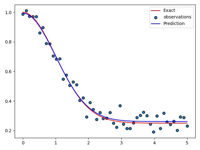
求解非线性模型$f(x,\beta )={\beta }_0+{\beta }_1{e}^{\left(-{\beta }_2{x}^2\right)}$，有一组观测值$\left(x_i,y_i\right)$

问题求解

利用scipy.optimize.leastsq函数求解最佳最小二乘拟合。

import numpy as np
from scipy.optimize import leastsq
import matplotlib.pyplot as plt
# Exact function
beta = (0.25, 0.75, 0.5)

def f(x, b0, b1, b2):
    return b0 + b1 * np.exp(-b2 * x ** 2)

def g(beta):
    res = (ydata - f(xdata, *beta))
    return res
# return res.shape = {tuple:1}, res ={ndarray:{(50,)}}

# noisy observation
xdata = np.linspace(0, 5, 50)
y = f(xdata, *beta)
ydata = y + 0.05 * np.random.randn(len(xdata))

beta_start = (1, 1, 1)
# beta_opt为优化的参数
beta_opt, beta_cov = leastsq(g, beta_start)

# Exact
xdata = np.linspace(0, 5, 50)
y = f(xdata, *beta)
plt.plot(xdata, y, 'r',label='Exact')
plt.scatter(xdata, ydata,s =None, edgecolors='k', label='observations')

# Predictions
xdata = np.linspace(0, 5, 50)
y_pred = f(xdata, *beta_opt)
plt.plot(xdata, y_pred, 'b',label='Prediction')
plt.legend()
plt.show()

结果展示

基于Jacobi矩阵的最小二乘求解方法

与上一个问题不同，该方法利用求解目标函数的梯度信息构建Jacobi矩阵进行求解${\theta }_1,{\theta }_2$ and $\varphi$。
利用optimize.least_squares()求解。

问题定义

all_phase $\times A\times B\times C=\left[\begin{array}{l}\alpha \\ \beta \end{array}\right]$，求解${\theta }_1,{\theta }_2$ , $\varphi$
其中，
$A=\frac{1}{\sqrt{2}}\left[\begin{array}{cc}1+i\cos 2{\theta }_1& i\sin 2{\theta }_1\\ i\sin 2{\theta }_1& 1-i\cos 2{\theta }_1\end{array}\right]$
$B=e^{i\frac{\pi }{2}}\left[\begin{array}{cc}\cos 2{\theta }_2& \sin 2{\theta }_2\\ \sin 2{\theta }_2& -\cos 2{\theta }_2\end{array}\right]$
$C=\left[\begin{array}{l}1\\ 0\end{array}\right]$
all_phase $=e^{i\varphi }$
$\left[\begin{array}{l}\alpha \\ \beta \end{array}\right]=\left[\begin{array}{c}\cos {\psi }_1\\ e^{i{\psi }_2}\sin {\psi }_1\end{array}\right]$
以及，${\theta }_1,{\theta }_2$ , $\varphi$为未知参数，${\theta }_1\in [0,\pi ),{\theta }_2\in [0,\pi ),\varphi \in [0,\pi )$，已知参数${\psi }_1$ and ${\psi }_2,{\psi }_1,{\psi }_2\in \mathcal{R}$。

问题求解

步骤：

• 计算Jacobi矩阵
• 利用optimize.least_squares()求解

详细步骤：

• 第一步，计算目标函数

# unknown parameters; to be solved
theta1 = sp.Symbol('theta1', real=True)
theta2 = sp.Symbol('theta2', real=True)
phi = sp.Symbol('phi', real=True)

# known hyperparameters; to be set
psi1 = sp.Symbol('psi1', real=True)  
psi2 = sp.Symbol('psi2', real=True)

alpha = sp.cos(psi1)   # real number
beta = sp.sin(psi1) * sp.exp(psi2 * 1j)  # complex number

# construct the matrices
x = theta1 * 2
y = theta2 * 2

# sumpy的 I 等于 python自带的 1j
A = sp.Matrix([[1 + 1j * sp.cos(x), 1j * sp.sin(x)], [1j * sp.sin(x), 1 - 1j * sp.cos(x)]]) * np.sqrt(1/2)
B = sp.Matrix([[sp.cos(y), sp.sin(y)],[sp.sin(y), - sp.cos(y)]]) * 1j
C = sp.Matrix([[1], [0]])
all_phase = sp.exp( phi*1j )
# 优化目标函数
D = A * B * C * all_phase
D1 = sp.simplify(D)

J1 = sp.simplify(sp.re(D1[0]) - sp.re(alpha))
J2 = sp.simplify(sp.im(D1[0]) - sp.im(alpha))
J3 = sp.simplify(sp.re(D1[1]) - sp.re(beta))
J4 = sp.simplify(sp.im(D1[1]) - sp.im(beta)

$D1=\left[\begin{array}{c}0.707106781186548\left(i\cos \left(2{\theta }_2\right)-\cos \left(2{\theta }_1-2{\theta }_2\right)\right)e^{1.0i\varphi }\\ 0.707106781186548\left(i\sin \left(2{\theta }_2\right)-\sin \left(2{\theta }_1-2{\theta }_2\right)\right)e^{1.0i\varphi }\end{array}\right]$

$\alpha ,\beta =\left(\cos \left({\psi }_1\right),e^{1.0i{\psi }_2}\sin \left({\psi }_1\right)\right)$

四个方程$J_1$,$J_2$,$J_3$,$J_4$分别为
$J_1=-0.707106781186548\sin (1.0\varphi )\cos \left(2{\theta }_2\right)-0.707106781186548\cos (1.0\varphi )\cos \left(2\left({\theta }_1-{\theta }_2\right)\right)-\cos \left({\psi }_1\right)$
$J_2=-0.707106781186548\sin (1.0\varphi )\cos \left(2\left({\theta }_1-{\theta }_2\right)\right)+0.707106781186548\cos (1.0\varphi )\cos \left(2{\theta }_2\right)$
$J3=-0.707106781186548\sin (1.0\varphi )\sin \left(2{\theta }_2\right)-\sin \left({\psi }_1\right)\cos \left(1.0{\psi }_2\right)-0.707106781186548\sin \left(2\left({\theta }_1-{\theta }_2\right)\right)\cos (1.0\varphi )$
$J4=-0.707106781186548\sin (1.0\varphi )\sin \left(2{\theta }_1-2{\theta }_2\right)-\sin \left({\psi }_1\right)\sin \left(1.0{\psi }_2\right)+0.707106781186548\sin \left(2{\theta }_2\right)\cos (1.0\varphi )$

• 计算Jacobi行列式

dJ1_theta1 = sp.simplify(sp.diff(J1, theta1))
dJ1_theta2 = sp.simplify(sp.diff(J1, theta2))
dJ1_phi = sp.simplify(sp.diff(J1, phi))

dJ3_theta1 = sp.simplify(sp.diff(J3, theta1))
dJ3_theta2 = sp.simplify(sp.diff(J3, theta2))
dJ3_phi = sp.simplify(sp.diff(J3, phi))

dJ4_theta1 = sp.simplify(sp.diff(J4, theta1))
dJ4_theta2 = sp.simplify(sp.diff(J4, theta2))
dJ4_phi = sp.simplify(sp.diff(J4, phi))

雅可比行列式的每一行，dJ1_theta1,dJ1_theta2,dJ1_phi, dJ3_theta1,dJ3_theta2,dJ3_phi,dJ4_theta1,dJ4_theta2,dJ4_phi

$\mathbf{J}=\left[\begin{array}{ccc}\frac{\partial \mathbf{f}}{\partial x_1}& \cdots & \frac{\partial \mathbf{f}}{\partial x_n}\end{array}\right]=\left[\begin{array}{ccc}\frac{\partial f_1}{\partial x_1}& \cdots & \frac{\partial f_1}{\partial x_n}\\ ⋮& \ddots & ⋮\\ \frac{\partial f_m}{\partial x_1}& \cdots & \frac{\partial f_m}{\partial x_n}\end{array}\right]$

• 代码实现

import sympy as sp
import numpy as np
from scipy import optimize
# x:[theta1, theta2, phi]; psi=pi/4
# f consists of [J1,J3,J4]
# 目标函数
def fun_tf_ls(x, psi1, psi2):
    f = [- np.sqrt(1 / 2) * np.sin(x[2]) * np.cos(2 * x[1])
         - np.sqrt(1 / 2) * np.cos(x[2]) * np.cos(2 * (x[0] - x[1])) - np.cos(psi1),

         - np.sqrt(1 / 2) * np.sin(x[2]) * np.sin(2 * x[1])
         - np.sqrt(1 / 2) * np.sin(2 * (x[0] - x[1])) * np.cos(x[2]) - np.sin(psi1) * np.cos(psi2),

         - np.sqrt(1 / 2) * np.sin(x[2]) * np.sin(2 * (x[0] - x[1]))
         + np.sqrt(1 / 2) * np.sin(2 * x[1]) * np.cos(x[2]) - np.sin(psi1) * np.sin(psi2)]  # 3个方程
    return f

# 雅可比行列式
def deri_tf_ls(x, psi1, psi2):
    df = np.array([[2 * np.sqrt(1 / 2) * np.sin(2 * (x[0] - x[1])) * np.cos(x[2]),
                    2 * np.sqrt(1 / 2) * (np.sin(x[2]) * np.sin(2 * x[1]) - np.sin(2 * (x[0] - x[1])) * np.cos(x[2])),
                    np.sqrt(1 / 2) * (np.sin(x[2]) * np.cos(2 * (x[0] - x[1])) - np.cos(x[2]) * np.cos(2 * x[1]))],
                   [-2 * np.sqrt(1 / 2) * np.cos(x[2]) * np.cos(2 * (x[0] - x[1])),
                    -2 * np.sqrt(1 / 2) * (np.sin(x[2]) * np.cos(2 * x[1]) - np.cos(x[2]) * np.cos(2 * (x[0] - x[1]))),
                    np.sqrt(1 / 2) * (np.sin(x[2]) * np.sin(2 * (x[0] - x[1])) - np.sin(2 * x[1]) * np.cos(x[2]))],
                   [-2 * np.sqrt(1 / 2) * np.sin(x[2]) * np.cos(2 * (x[0] - x[1])),
                    2 * np.sqrt(1 / 2) * (np.sin(x[2]) * np.cos(2 * (x[0] - x[1])) + np.cos(x[2]) * np.cos(2 * x[1])),
                    -np.sqrt(1 / 2) * (np.sin(x[2]) * np.sin(2 * x[1]) + np.cos(x[2]) * np.sin(2 * (x[0] - x[1])))]
                   ])  # 3 X 3
    return df
psi1_0 = np.pi / 4
psi2_0 = np.pi / 2
x0 = np.array([1, 1, 1])
# 限定[theta1, theta2, phi]的定义域为[0,pi]
# bounds=(lower_bound, upper_bound); 
# lower_bound和upper_bound可以为具体数值，也可以为np.inf（正无穷或-np.inf(负无穷)
# 给每个自变量单独指定定义域：bounds=([0,0,0], [np.pi, np.pi, np.pi])
# 为所有自变量指定相同的定义域: bounds=(0,np.pi)
sol_tf = optimize.least_squares(fun_tf_ls, x0, args=(psi1_0,psi2_0), jac=deri_tf_ls, bounds=(0, np.pi))
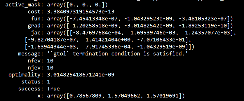
print(sol_tf)
# sol_tf.x为优化结果，sol_tf.cost为优化目标损失值，sol_tf.fun为目标函数值

结果为

此外，特别注意的是，需先将Jacobi形式计算出。若deri_tf_ls(x, psi1, psi2)函数中是关于x的变量求导，如下

def deri_tf_ls(c):
    f_sym = target
    J = [J_ for J_ in f_sym]
    J_obj = J
    J_dc = np.array([[sp.diff(J_, c_) for J_ in J] for c_ in c]).T  # 雅克比矩阵

其中，diff是对自变量c求导，但是调用least_squares函数输入的c为具体的值。就会报错

参考

https://blog.csdn.net/sinat_21591675/article/details/85936621
https://zhuanlan.zhihu.com/p/101645294