文章目录
任务:利用INRIA Person数据集,提取HOG特征并采用SVM方法实现图像中的行人检测。
本文将给出详细的操作步骤,以及可能会出现的坑点。
一、准备工作
1. 下载数据集
INRIA数据集含有直立或行走的人的图像,被Navneet Dalal用于训练发表在CVPR 2005的人类检测器。
坑点1:官网http://pascal.inrialpes.fr/data/human/打开后显示403 Forbidden。
解决方法:使用Motrix/IDM/迅雷(或其他支持FTP的下载工具)打开ftp://ftp.inrialpes.fr/pub/lear/douze/data/INRIAPerson.tar进行下载(压缩后大小1GB左右)。
2. 解压数据集
坑点2:使用WinRAR/7Zip解压时出现文件覆盖、要求管理员权限等问题。
解决方法:文件中含有软连接,不能使用WinRAR/7Zip解压,而应使用来自Linux的命令tar解压。如果你安装了WSL(Windows Subsystem for Linux)/MinGW等类Linux环境,可以调用如下命令:
tar xvf INRIAPerson.tar
其中x代表Extract(解压),v代表Verbose(显示正在解压的文件),f代表File Name(后面跟文件名)。这个命令将会在当前目录下生成INRIAPerson文件夹,里面是解压的文件。
二、HOG特征简介
HOG的全称是方向梯度直方图(Histogram of Oriented Gradient),它是计算机视觉中用于物体检测的一种特征描述子(Feature Descriptor)。特征描述子的作用是提取有用的信息,抛弃冗余的信息。对于一个物体而言,能够区分它的特征的往往是它的形状——也就是它的边界。而在边界处灰度一般有突变,所以我们考察图像的梯度就可以知道边界在什么地方。
1. 梯度(Gradient)
首先,我们假设输入图片是一张灰度图(其实我们一般处理的是图像的一部分,即window,而不是整个图像)。它可以看作是行( r r r)和列( c c c)的二元函数: I ( r , c ) I(r,c) I(r,c),其中 I I I代表第 r r r行、 c c c列的像素点的灰度(取值范围为 0 0 0~ 255 255 255)。在研究二元函数时,我们常常会考虑它的梯度。在这里,我们需要知道 I I I在 x x x、 y y y方向的梯度。我们采取的办法是:使用相邻格子的灰度之差做近似。 I I I在 x x x、 y y y方向的梯度公式如下: I x ( r , c ) = I ( r , c + 1 ) − I ( r , c − 1 ) I y ( r , c ) = I ( r + 1 , c ) − I ( r − 1 , c ) \begin{aligned} I_x(r,c)&=I(r,c+1)-I(r,c-1)\\ I_y(r,c)&=I(r+1,c)-I(r-1,c) \end{aligned} Ix(r,c)Iy(r,c)=I(r,c+1)−I(r,c−1)=I(r+1,c)−I(r−1,c)按理来说,上面的式子应该都除以 2 2 2,但因为后面要做归一化处理,所以这些常数就无关紧要了。它也可以理解为用向量 [ − 1 0 1 ] \begin{bmatrix}-1&0&1\end{bmatrix} [−101]和 [ − 1 0 1 ] {\begin{bmatrix}-1\\0\\1\end{bmatrix}} −101 对原图做卷积运算。接下来我们把梯度转换为极坐标,其中角度被限制在 0 ° 0\degree 0°~ 180 ° 180\degree 180°: μ = I x 2 + I y 2 θ = 180 π ( arctan I y I x ) \begin{aligned} \mu&=\sqrt{I_x^2+I_y^2}\\ \theta&=\frac{180}{\pi}\left(\arctan\frac{I_y}{I_x}\right) \end{aligned} μθ=Ix2+Iy2=π180(arctanIxIy)这里我们把 arctan \arctan arctan定义为 arctan x = { tan − 1 x , x ≥ 0 tan − 1 x + π , x < 0 \arctan x=\begin{cases} \tan^{-1}x,&x\ge 0\\ \tan^{-1}x+\pi,&x<0 \end{cases} arctanx={ tan−1x,tan−1x+π,x≥0x<0并且 θ \theta θ用角度制表示。
2. 格子(Cell)
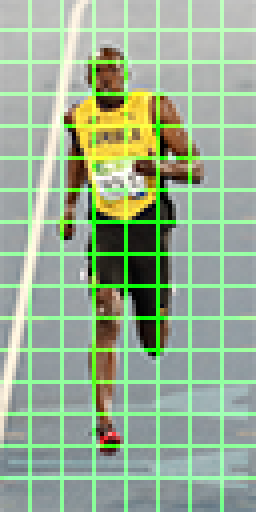
我们继续将图像分割为 C × C C\times C C×C大小的格子(一般 C = 8 C=8 C=8)。下图演示了这样的一个分割,每个绿框是 8 × 8 8\times 8 8×8大小的格子:
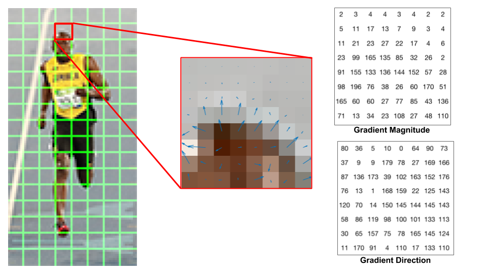
每个格子有 C 2 C^2 C2(一般为 64 64 64)个像素点。每个像素点有一个梯度,我们要统计这些像素点梯度方向(即角度 θ \theta θ)的分布规律。上图中某个格子的梯度模长、方向如下:
想要统计角度的分布规律,就要用到直方图(Histogram)的概念了。在直方图中, x x x轴的每个区间称为一个bin,你可以把bin理解为桶,输入数据根据它在哪个范围里面被放进对应的桶里。那么对于 θ \theta θ,它的范围是 0 ° 0\degree 0°~ 180 ° 180\degree 180°,我们这个范围分成 B B B个bin。一般取 B = 9 B=9 B=9,也就是说每个区间的宽度是 w = 180 B = 20 ° w=\frac{180}{B}=20\degree w=B180=20°。我们把每个bin从 0 0 0到 B − 1 B-1 B−1进行编号。第 i i i个bin的范围是 [ w i , w ( i + 1 ) ) [wi,w(i+1)) [wi,w(i+1)),中心是 w ( i + 1 2 ) w\!\left(i+\frac{1}{2}\right) w(i+21)。例如,当 B = 9 B=9 B=9时,第3个bin( i = 3 i=3 i=3)的范围是 [ 60 ° , 80 ° ) [60\degree,80\degree) [60°,80°),中心是 70 ° 70\degree 70°。但是呢,我们不会简单的把每个像素点根据 θ \theta θ所在的范围放进桶里,而是需要考虑 μ \mu μ的大小,把它按一定比例放进相邻的两个桶里。最后,每个桶的值其实不是个数,而是一种“贡献”(contribution)的度量。一个像素点对一个bin的贡献不仅取决于梯度的模长 μ \mu μ,还取决于它的角度 θ \theta θ与该bin的中心的距离。模长越长,贡献越大;距离越远,贡献越小。具体地说,对于一个梯度模长为 μ \mu μ、方向角为 θ \theta θ的像素点,设 j = ⌊ θ w − 1 2 ⌋ j=\left\lfloor\cfrac{\theta}{w}-\cfrac{1}{2}\right\rfloor j=⌊wθ−21⌋,则它

- 对编号为 j m o d b j\bmod b jmodb的bin的贡献为 v j = μ c j + 1 − θ w v_j=\mu\cfrac{c_{j+1}-\theta}{w} vj=μwcj+1−θ;
- 对编号为 ( j + 1 ) m o d b (j+1)\bmod b (j+1)modb的bin的贡献为 v j + 1 = μ θ − c j w v_{j+1}=\mu\cfrac{\theta-c_j}{w} vj+1=μwθ−cj。
最后,每个格子会得到一个直方图,直方图的每个条目是所有这个格子中的像素点对这个bin的贡献之和。有趣的是,每个像素点对两个bin的贡献之和一定是 μ \mu μ。
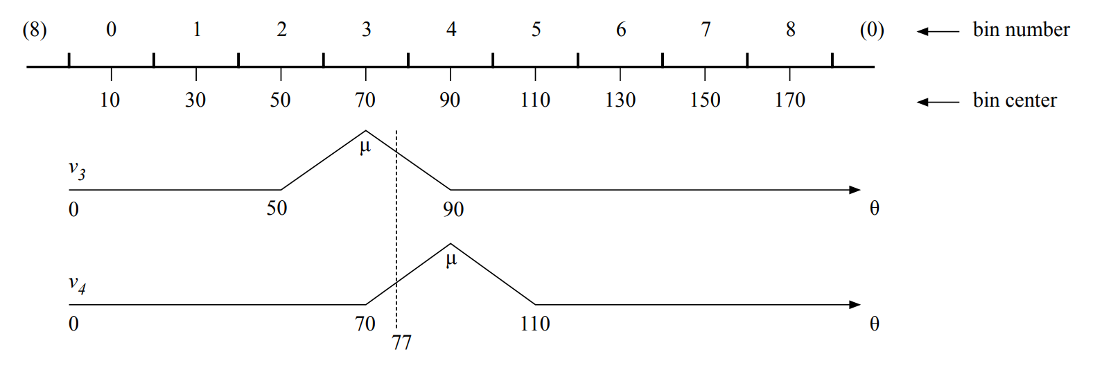
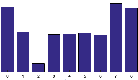
下图是一个例子。首先,我们把 0 ° 0\degree 0°~ 180 ° 180\degree 180°分成 B = 9 B=9 B=9份,每一份的中心分别为 10 ° 10\degree 10°、 30 ° 30\degree 30°、…、 170 ° 170\degree 170°。现在我们有一个 θ = 77 ° \theta=77\degree θ=77°、模长为 μ \mu μ的梯度,它对3号bin(范围是 60 ° 60\degree 60°~ 80 ° 80\degree 80°、中心为 70 ° 70\degree 70°)的贡献为 0.65 μ 0.65\mu 0.65μ,对4号bin(范围是 80 ° 80\degree 80°~ 100 ° 100\degree 100°、中心为 90 ° 90\degree 90°)的贡献为 0.35 μ 0.35\mu 0.35μ。
对于运动员的那张图,下图展示了如何计算一个梯度模长为 85 85 85、角度为 165 165 165的像素点的贡献:
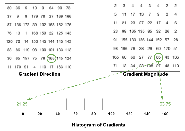
这个格子的直方图如下:
3. 块归一化(Block Normalization)
虽然我们已经获得了一个直方图,但是整体而言,直方图的高度与图像的亮度有很大关系,我们不希望白天拍的照片和晚上拍的照片整体的直方图高度差距很大。于是乎,我们需要对其进行归一化。把格子打包成块(block),每块有 2 × 2 2\times 2 2×2个格子,且块之间是可以重合的。显然,每块包含像素点的个数为 2 C × 2 C 2C\times 2C 2C×2C。我们按照滑动窗口的方式把整个window扫描一遍,每次移动一个块。这样就保证了每个不在边缘的格子都被四个块覆盖。
上图的大小为 64 × 128 64\times 128 64×128,即 8 × 16 8\times 16 8×16个格子,每个块的水平位置有 7 7 7个,竖直位置有 15 15 15个。
现在,既然每个块有 4 4 4个格子,每个格子的直方图有 9 9 9个条目,我们可以把这些直方图的条目连接起来,形成 36 36 36维的向量 b \boldsymbol{b} b。现在,我们利用欧几里得范数(Euclidean norm)把每个块的 b \boldsymbol{b} b归一化,使其模长接近于 1 1 1: b : = b ∥ b ∥ 2 + ε \boldsymbol{b}:=\frac{\boldsymbol{b}}{\sqrt{ {\|\boldsymbol{b}\|}^2+\varepsilon}} b:=∥b∥2+εb其中 ε \varepsilon ε是为了防止除以 0 0 0加上的一个非常小的正数。
你可能会问:为什么不对每个格子进行归一化呢?答案是,格子之间直方图高度的整体差异是携带了一部分信息的,不能把这部分信息彻底抹去。而对每个 2 × 2 2\times 2 2×2的块进行归一化,可以在一定程度上保留不同格子之间平均灰度差异所代表的信息。
4. HOG特征(HOG Feature)
接下来,我们把每个块的 b \boldsymbol{b} b向量全部连接起来,形成一个巨大的向量 h \boldsymbol{h} h,然后进行如下三步操作:
(1) 进行一个初步的归一化: h : = h ∥ h ∥ 2 + ε \boldsymbol{h}:=\cfrac{\boldsymbol{h}}{\sqrt{ {\|\boldsymbol{h}\|}^2+\varepsilon}} h:=∥h∥2+εh;
(2) 使得 h \boldsymbol{h} h中每个数的大小不超过一个正的阈值 τ \tau τ,即对 h \boldsymbol{h} h的第 n n n维 h n h_n hn,令 h n : = min ( h n , τ ) h_n:=\min(h_n,\tau) hn:=min(hn,τ);
(3) 最后再进行一次归一化: h : = h ∥ h ∥ 2 + ε \boldsymbol{h}:=\cfrac{\boldsymbol{h}}{\sqrt{ {\|\boldsymbol{h}\|}^2+\varepsilon}} h:=∥h∥2+εh。这样我们就大功告成啦。
对于一个 Y Y Y行、 X X X列的window,它的格子数是 Y C × X C \cfrac{Y}{C}\times\cfrac{X}{C} CY×CX,块数是 ( Y C − 1 ) × ( X C − 1 ) \left(\cfrac{Y}{C}-1\right)\times\left(\cfrac{X}{C}-1\right) (CY−1)×(CX−1),最后HOG特征 h \boldsymbol{h} h的维数是 4 B × ( Y C − 1 ) × ( X C − 1 ) 4B\times\left(\cfrac{Y}{C}-1\right)\times\left(\cfrac{X}{C}-1\right) 4B×(CY−1)×(CX−1)。那张运动员图片的HOG特征维数是 4 × 9 × 15 × 7 = 3780 4\times 9\times 15\times 7=3780 4×9×15×7=3780。
5. 使用skimage.feature.hog提取HOG特征
skimage的安装方法:
pip install -i https://pypi.tuna.tsinghua.edu.cn/simple scikit-image
对于这张 96 × 160 96\times 160 96×160的图片(名为hog_test.png)

下面的代码提取了它的HOG特征:
# encoding: UTF-8
# 文件: hog.py
# 描述: 提取图片的HOG特征

from skimage.io import imread
from skimage.feature import hog

def extract_hog_feature(filename):
    # 提取filename文件的HOG特征
    image = imread(filename, as_gray=True)
    # 读取图片,as_gray=True表示读取成灰度图
    feature = hog( # 提取HOG特征
        image, # 图片
        orientations=9, # 方向的个数,即bin的个数B
        pixels_per_cell=(8, 8), # 格子的大小,C×C
        cells_per_block=(2, 2), # 一块有2×2个格子
        block_norm='L2-Hys', # 归一化方法
        visualize=False # 是否返回可视化图像
    )
    return feature

if __name__ == '__main__':
    feature = extract_hog_feature('hog_test.png')
    print(feature) # 显示HOG特征
    print(feature.shape) # 显示HOG特征的维数
输出结果为:
[0.24284172 0.24284172 0.21779826 ... 0.1942068  0.25568547 0.10666346]
(7524,)
也就是说,我们获得的HOG特征是一个 7524 7524 7524维的向量。此处 7524 = 4 × 9 × ( 96 8 − 1 ) × ( 160 8 − 1 ) 7524=4\times 9\times\left(\cfrac{96}{8}-1\right)\times\left(\cfrac{160}{8}-1\right) 7524=4×9×(896−1)×(8160−1)。
如果我们把visualize设置为True,则hog函数会返回一个包含HOG特征和可视化图片的元组,调用
import matplotlib.pyplot as plt
...
feature, visimg = hog(...)
plt.imshow(visimg)
plt.show()
得
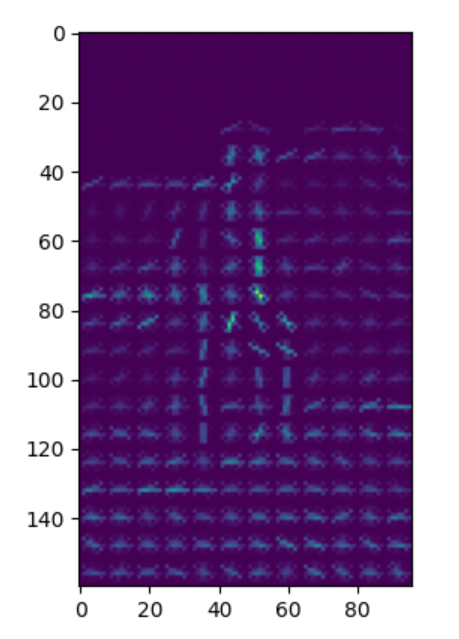
这就是图片hog_test.png的HOG特征的可视化。
6. 总结
现在我们把一个图片利用HOG特征转化成了一个向量,接下来就可以利用SVM分类了。
三、支持向量机模型的训练和测试
在支持向量机(Support Vector Machine, SVM)基础知识这篇文章中我们介绍了SVM的基本原理。接下来我主要介绍SVM的Python实现。
1. 处理数据集
训练数据集
按理来说,训练数据的正样本(有人的图片)放在INRIAPerson\train_64x128_H96\pos文件夹里面,负样本(没人的图片)放在INRIAPerson\train_64x128_H96\neg文件夹里面,并且图片应该是 64 × 128 64\times 128 64×128大小的。不过,事实并不是这样:
坑点3:INRIAPerson\train_64x128_H96\pos文件夹里面没有图片,只有软连接;INRIAPerson\train_64x128_H96\neg直接就是一个软连接。并且,pos连接到的是INRIAPerson\96X160H96\Train\pos里面的文件,这些图片都是 96 × 160 96\times 160 96×160大小的;neg连接到的是INRIAPerson\Train\neg里面的文件,图片大小不一。
解决方法:
- 将
INRIAPerson\96X160H96\Train\pos作为正样本的文件夹,其中图片大小为 96 × 160 96\times 160 96×160的原因是图像周边有 16 × 16 16\times 16 16×16的padding。所以读取图片时需截取中心 64 × 128 64\times 128 64×128大小的部分,即坐标为 ( 16 , 16 ) (16,16) (16,16)~ ( 80 , 144 ) (80,144) (80,144)的部分。 - 将
INRIAPerson\Train\neg作为负样本的文件夹,并且对于每个图片我们随机截取 10 10 10个 64 × 128 64\times 128 64×128的部分。
测试数据集
同理,将INRIAPerson\70X134H96\Test\pos作为测试正样本的文件夹,INRIAPerson Test\neg为测试负样本的文件夹。
2. 读取图片、提取HOG特征
由于数据量过大,每格包含像素点个数 C C C取 8 8 8时会导致训练极慢,所以这里我取 C = 16 C=16 C=16。
对于正样本,我们截取器中间 64 × 128 64\times 128 64×128大小的部分,提取其HOG特征。对于负样本,我们在上面随机截取 10 10 10个 64 × 128 64\times 128 64×128的部分,提取HOG特征。最后得到两个列表:x和y,其中x是HOG特征(即训练数据),y是标签,若x[i]来自正样本则y[i] = 1,否则y[i] = 0。代码如下:
import random
import os
import tqdm # 用于在循环时显示进度条
from skimage.io import imread # 读取图像的函数
from skimage.feature import hog # skimage自带的提取HOG特征的函数

def clip_image(img, left, top,
    width=64, height=128):
    '''
    截取图片的一个区域。

    参数
    ---
    img: 图片输入。
    left: 区域左边的坐标。
    top: 区域上边的坐标。
    width: 区域宽度。
    height: 区域高度。
    '''
    return img[top:top + height, left:left + width]

def extract_hog_feature(img):
    '''
    提取单个图像img的HOG特征。
    '''
    return hog(
        img,
        orientations=9,
        pixels_per_cell=(16, 16),
        cells_per_block=(2, 2),
        block_norm='L2-Hys',
        visualize=False
    ).astype('float32')

def read_images(pos_dir, neg_dir,
    neg_area_count, description):
    '''
    读取图片,提取样本HOG特征。

    参数
    ---
    pos_dir: 正样本所在文件夹。
    neg_dir: 负样本所在文件夹。
    neg_area_count: 在每个负样本中随机截取区域的个数。
    description: 用途描述(训练/测试)。

    返回值
    -----
    返回一个元组(x, y),x是所有图片的HOG特征,
    y是所有图片的分类(1=正样本,0=负样本)。
    '''
    pos_img_files = os.listdir(pos_dir)
    # 正样本文件列表
    neg_img_files = os.listdir(neg_dir)
    # 负样本文件列表

    area_width = 64 # 截取的区域宽度
    area_height = 128 # 截取的区域高度

    x = [] # 图片的HOG特征
    y = [] # 图片的分类

    for pos_file in tqdm(pos_img_files,
        desc=f'{

      description}正样本'):
        # 读取所有正样本
        pos_path = os.path.join(pos_dir, pos_file)
        # 正样本路径
        pos_img = imread(pos_path, as_gray=True)
        # 正样本图片
        img_height, img_width = pos_img.shape
        # 该图片的宽、高
        clip_left = (img_width - area_width) // 2
        # 截取区域的左边
        clip_top = (img_height - area_height) // 2
        # 截取区域的上边
        pos_center = clip_image(pos_img,
            clip_left, clip_top, area_width, area_height)
        # 截取中间部分
        hog_feature = extract_hog_feature(
            pos_center) # 提取HOG特征
        x.append(hog_feature) # 加入HOG向量
        y.append(1) # 1代表正类

    for neg_file in tqdm(neg_img_files,
        desc=f'{

      description}训练负样本'):
        # 读取所有负样本
        neg_path = os.path.join(neg_dir, neg_file)
        # 负样本路径
        neg_img = imread(neg_path, as_gray=True)
        # 负样本图片
        img_height, img_width = neg_img.shape
        # 该图片的宽、高
        left_max = img_width - area_width
        # 区域左边坐标的最大值
        top_max = img_height - area_height
        # 区域
        for _ in range(neg_area_count):
            # 随机截取neg_area_count个区域
            left = random.randint(0, left_max) # 区域左边
            top = random.randint(0, top_max) # 区域上边
            clipped_area = clip_image(neg_img,
                left, top, area_width, area_height)
            # 截取的区域
            hog_feature = extract_hog_feature(
                clipped_area) # 提取HOG特征
            x.append(hog_feature)
            y.append(0)
    return x, y
上面的read_images函数既可用于读取训练数据,也可用于读取测试数据。
坑点4:skimage.io.imread读出来的图像是“高×宽”形式的,而不是“宽×高”形式的。
解决方法:在截取图片时注意,下标的第一维是纵坐标,第二维是横坐标。
下面的两个函数read_training_data和read_test_data调用read_images函数分别读取训练数据和测试数据(返回值仍然是两个:HOG特征和标签)。不论是训练还是测试数据,负样本均随机截取10个区域。
def read_training_data():
    '''
    读取训练数据。
    '''
    pos_dir = 'INRIAPerson/96X160H96/Train/pos'
    neg_dir = 'INRIAPerson/Train/neg'
    neg_area_count = 10
    description = '训练'
    return read_images(pos_dir, neg_dir,
        neg_area_count, description)

def read_test_data():
    '''
    读取测试数据。
    '''
    pos_dir = 'INRIAPerson/70X134H96/Test/pos'
    neg_dir = 'INRIAPerson/Test/neg'
    neg_area_count = 10
    description = '测试'
    return read_images(pos_dir, neg_dir,
        neg_area_count, description)
如果我们需要训练多次,我们不需要每次执行程序都提取图像的HOG特征。我们可以把已经算出来的HOG特征保存在文件里,在训练SVM时把数据从文件里面读取出来就可以了。保存和读取文件的函数如下:
def save_hog(x, y, filename):
    '''
    把read_training_samples的返回值(x, y)
    写入名为filename的文件。
    '''
    with open(filename, 'wb') as file:
        pickle.dump((x, y), file)

def load_hog(filename):
    '''
    从名为filename的文件中加载训练数据(x, y)。
    '''
    result = None
    with open(filename, 'rb') as file:
        result = pickle.load(file)
    return result
3. 训练SVM
在成功读取了训练数据之后,就要进入到训练SVM的环节了。SVM原理的介绍请参见支持向量机(Support Vector Machine, SVM)基础知识,这里我们调库就可以了。
sklearn中的SVM分类器类是sklearn.svm.SVC:
from sklearn.svm import SVC
我们重点关注SVC的几个参数。
tol:即“tolerance”。SVM的优化问题有一个条件:对于每个 i ( 1 ≤ i ≤ n ) i(1\le i\le n) i(1≤i≤n), y i ( w T x + b ) ≥ 1 y_i\left(\bm{w}^{\mathrm{T}}\bm{x}+b\right)\ge 1 yi(wTx+b)≥1。但对于非线性可分的数据,这个条件可能并不会永远被满足,所以我们把条件改的松一些,即 y i ( w T x + b ) ≥ 1 − ε y_i\left(\bm{w}^{\mathrm{T}}\bm{x}+b\right)\ge 1-\varepsilon yi(wTx+b)≥1−ε,其中 ε \varepsilon ε就是tol。tol越小,条件越严格。sklearn的默认tol是1e-3,我采用1e-6,使分类更严格一些。C:惩罚系数。对于非线性可分的样本,我们必须允许一些样本不满足约束条件,此时我们引入松弛变量 ξ i \xi_i ξi,将第 i i i个样本的限制条件从 y i ( w T x + b ) ≥ 1 − ε y_i\left(\bm{w}^{\mathrm{T}}\bm{x}+b\right)\ge 1-\varepsilon yi(wTx+b)≥1−ε改成 y i ( w T x + b ) ≥ 1 − ε − ξ i y_i\left(\bm{w}^{\mathrm{T}}\bm{x}+b\right)\ge 1-\varepsilon-\xi_i yi(wTx+b)≥1−ε−ξi,并且 ξ i ≥ 0 \xi_i\ge 0 ξi≥0。同时,优化的目的也应发生变化,我们希望不满足约束的变量个数越少越好,所以将优化目的改为 min w , b 1 2 ∥ w ∥ 2 + C ∑ i = 1 n ξ i \min\limits_{\bm{w},b}\frac{1}{2}{\|\bm{w}\|}^2+C\sum\limits_{i=1}^n\xi_i w,bmin21∥w∥2+Ci=1∑nξi,其中 C C C就是惩罚系数。惩罚系数体现了对不满足约束的变量的惩罚力度, C C C越大,对不满足约束的变量的容忍度越低。根据Dalal的论文(参考文献[6]),当 C = 0.01 C=0.01 C=0.01时取得了较好的结果,因此我也选取C = 0.01。max_iter:最大迭代次数。我们希望SVM达到目标情况时再结束迭代,所以将其设置为-1,代表不设置次数限制。gamma:高斯核的gamma参数,我们设置为auto,即自动设置gamma的值。kernel:核函数。根据Dalal的论文,采用高斯核对识别准确率有一定程度的提高,同时性能可能有所下降(相较于线性核而言),因此我采用高斯核(kernel = rbf)。probability:是否输出概率。在行人检测任务中,我们希望直到图片上一个区域有行人的概率,因此设置probability = True。
训练SVM的代码如下:
def train_SVM(x, y):
    '''
    训练SVM。

    参数
    ---
    x, y: read_training_samples的返回值。

    返回值
    -----
    返回训练所得的SVM。
    '''
    SVM = SVC(
        tol=1e-6,
        C=0.01,
        max_iter=-1,
        gamma='auto',
        kernel='rbf',
        probability=True
    ) # 创建SVM实例
    SVM.fit(x, y) # 进行训练
    return SVM
这里SVM也可以换成Logistic Regression模型,把SVM = SVC(...)换成LR = sklearn.linear_model.LogisticRegression(tol=1e-6, C=0.01, max_iter=10000)即可。
4. 测试SVM
在训练完成之后,我们需要利用测试数据对SVM进行测试。对于一个给定的样本,SVM给出的预测结果可能是正确的,也可能是错误的。如果SVM把正样本说成是含有人的,则称该样本为真正例(true positive, TP);如果把正样本说成是不含人的,则称为假反例(false negative, FN);如果把负样本说成是含有人的,则称为假正例(false positive, FP);如果把负样本说成是不含人的,则称为真反例(true negative, TN)。其中,真正例和真反例是预测正确的情况,假正例和假反例是预测错误的情况。可以汇总成表格如下:
| 真实值 \ SVM分类结果 | 正 | 负 |
|---|---|---|
| 正 | 真正例(TP) | 假反例(FN) |
| 负 | 假正例(FP) | 真反例(TN) |
正样本(即真实值为正)的个数为TP+FN,负样本的个数为FP+TN。
定义查全率(Recall)为正样本中预测为正的比例,即Recall=TP/(TP+FN);查准率(Precision)为SVM说是正的样本中真的是正样本的比例,即Precision=TP/(TP+FP)。查全率还有一个名字,叫做真阳性率(True Positive Rate, TPR),与之相应的还有假阳性率(False Positive Rate, FPR),是负样本中预测为正的样本比例,即FPR=FP/(FP+TN)。显然FPR=1-TPR。定义缺失率(Miss Rate, MR)为正样本中没有查出来的比例,即MR=1-Recall=FN/(TP+FN)。
SVM的输出结果是图片的一个区域中含有行人的概率,我们定义一个阈值(threshold),使得如果SVM给出的概率大于等于该阈值,则认为该区域中有行人(即预测结果为正);如果概率小于该阈值,则认为该区域中没有行人(即预测结果为负)。阈值不同,预测结果也就不同。当阈值接近 1 1 1时,SVM预测结果为正的条件及其苛刻,真正例和假正例都有所减少,而假反例和真反例增加;反之,当阈值接近 0 0 0时,SVM会将很多样本说成是有行人的,真正例和假正例有所增加,而假反例和真反例减少。由于TP+FN和FP+TN不变,因此,阈值越大,Miss Rate越大(因为FN增大),而FPR减少(因为FP减少)。这样,对于每一个阈值,我们可以获得一个Miss Rate和一个FPR。将阈值取遍SVM对每个测试样本给出的不同的概率,我们可以画出一个Miss Rate-False Positive Rate曲线:
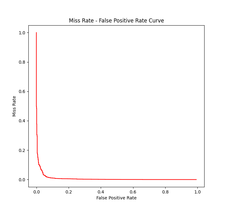
该曲线越靠近坐标轴(即曲线下面积越小),模型越可靠。这是因为,Miss Rate和False Positive Rate都是我们希望减少的量,我们希望它们同时取较小的值,也就是说,给定Miss Rate的值,False Positive Rate越小越好,即曲线下面积越小越好。
我们用函数test_SVM对SVM进行测试。首先调用SVM.predict_proba方法计算出每个测试样本含有行人的概率,然后计算对于每个阈值Miss Rate和False Positive Rate的值,画出Miss Rate-False Positive Rate曲线。最后,函数返回ROC曲线(Receiver Operating Characteristic Curve)的曲线下面积(Area Under the Curve, AUC)值,该值越接近 1 1 1说明模型越可靠。
import numpy as np
import matplotlib.pyplot as plt
from sklearn import metrics

def test_SVM(SVM, test_data, show_stats=False):
    '''
    测试训练好的SVM。

    参数
    ---
    SVM: 训练好的SVM模型。
    test_data: 测试数据(read_test_data的返回值)。
    show_stats: 是否显示统计数据(miss rate vs.
    false positive rate曲线)。

    返回值
    -----
    返回AUC(ROC曲线下的面积)。AUC介于0.5和1之间。
    AUC越接近1,模型越可靠。
    '''
    hog_features = test_data[0] # 测试数据的HOG特征
    labels = test_data[1] # 数据标签(0=不是人,1=是人)
    prob = SVM.predict_proba(hog_features)[:, 1]
    if show_stats:
        # 下面将prob和labels按prob的降序排序
        sorted_indices = np.argsort(
            prob, kind="mergesort")[::-1]
        labels = labels[sorted_indices]
        prob = prob[sorted_indices]
        distinct_value_indices = np.where(np.diff(prob))[0]
            # prob中不同值第一次出现的下标
        threshold_idxs = np.r_[
            distinct_value_indices, labels.size - 1]
            # 阈值的下标,在末尾增加了最后一个样本的下标
        tps = np.cumsum(labels)[threshold_idxs]
            # 不同概率阈值对应的真正例数。
            # 注意现在已经按prob的降序排序,
            # 这种写法正确的原因是:在数组某一位置前的概率
            # 一定大于阈值,在此之后的概率一定小于阈值,
            # 所以真正例数就是在这一位置之前的正样本数。
        fps = 1 + threshold_idxs - tps
            # 不同概率阈值对应的假正例数。
            # threshold_idxs存储的是下标,
            # 加一后变成个数,
            # 再减去真正例数就是假正例数。
        num_positive = tps[-1]
            # tps的最后一项就是labels的和,
            # 因此代表正例的个数。
        recall = tps / num_positive
            # 查全率就是在所有正例中查出了多少真正例。
        miss = 1 - recall # 计算miss
        num_negative = fps[-1] # 负例个数
        fpr = fps / num_negative
            # 假阳性率(false positive rate)
        plt.plot(miss, fpr, color='red')
        plt.xlabel('False Positive Rate')
        plt.ylabel('Miss Rate')
        plt.title('Miss Rate - '
            'False Positive Rate Curve')
        plt.show()
    AUC = metrics.roc_auc_score(labels, prob)
    return AUC
5. 图像画框
接下来我们介绍在一个图像中框出行人的方法。主要的思想是滑动窗口(Sliding Windows)。即:采用大小不一的窗口在图像上以不同的步长滑过一遍,每次求出窗口中步长的HOG特征。算法有三层循环:
- 第一层枚举窗口的宽度。窗口的长宽比是固定的(2:1),宽度从一个初始的
min_width(默认为 48 48 48)开始,每次乘以width_scale(默认为 1.25 1.25 1.25)倍,当超过图像宽度时停止。如果你希望取得更好的识别效果,可以将min_width和width_scale设置的小一点,代价是识别速度会变慢。 - 第二层枚举窗口左侧的横坐标,从 0 0 0开始,每次增加一个步长
coord_step(默认为 16 16 16),直到右侧达到图像边界为止。如果你希望取得更好的识别效果,可以将coord_step调小,但识别速度仍然会变慢。 - 第三层枚举窗口上侧的纵坐标,从 0 0 0开始,每次增加一个步长
coord_step。 - 对于每个窗口,将其缩放成
area_width * area_height(默认为 64 × 128 64\times 128 64×128)的区域,提取其HOG特征。
然后,对于所有窗口的HOG特征,用SVM给出其中有行人的概率。当概率大于阈值threshold(默认为 0.99 0.99 0.99)时,视为有行人。但还有一个问题,一个行人可能会被多个方框框起来,我们需要选出其中最合适的方框。这就需要用到非极大值抑制(Non-Maximum Suppression, NMS)。

NMS的基本思想是,对于两个重叠部分较多的方框,舍弃其中含行人概率较小的那一个,保留概率较大的哪一个。怎么衡量重叠部分的多少呢?我们采用交并比(Intersection over Union, IoU)。IoU就是两个方框交集面积与并集面积的比值。IoU越大,重叠部分越多。当IoU大于等于一个阈值IoU_threshold时,则舍弃其中一个方框。
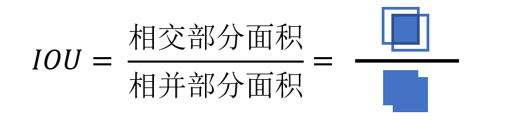
计算并集面积时只需要将两个方框面积相加再减去交集面积即可(类似于容斥原理)。代码如下:
def area_of_box(box):
    '''
    计算框的面积。

    参数
    ---
    box: 框,格式为(left, top, width, height)。

    返回值
    -----
    box的面积,即width * height。
    '''
    return box[2] * box[3]

def intersection_over_union(box1, box2):
    '''
    两个框的交并比(IoU)。

    参数
    ---
    box1: 边框1。
    box2: 边框2。
    '''
    intersection_width = max(0,
        box1[0] + box1[2] - box2[0])
        # 相交部分宽度=max(0, box1的右边 - box2的左边)
    intersection_height = max(0,
        box1[1] + box1[3] - box2[1])
        # 相交部分长度=max(0, box1的下边 - box2的上边)
    intersection_area = intersection_width * \
        intersection_height # 相交部分面积
    area_box1 = area_of_box(box1) # box1的面积
    area_box2 = area_of_box(box2) # box1的面积
    union_area = area_box1 + area_box2 - \
        intersection_area
    if abs(union_area) < 1:
        IoU = 0 # 防止除以0
    else:
        IoU = intersection_area / union_area
            # 并集的面积等于二者面积之和减去交集的面积
    return IoU
NMS算法的主要流程是:遍历每一个方框,如果它被另一个方框舍弃,则不加入结果列表,否则加入结果列表。最后返回结果列表。代码如下:
def non_maximum_suppression(pos_box_list, pos_prob,
    IoU_threshold=0.4):
    '''
    非极大值抑制(NMS)。

    参数
    ---
    pos_box_list: 含有人的概率大于阈值的边框列表。
    pos_prob: 对应的概率。
    IoU_threshold: 舍弃边框的IoU阈值。

    返回值
    -----
    抑制后的边框列表。
    '''
    result = [] # 结果
    for box1, prob1 in zip(pos_box_list, pos_prob):
        discard = False # 是否舍弃box1
        for box2, prob2 in zip(
            pos_box_list, pos_prob):
            if intersection_over_union(
                box1, box2) > IoU_threshold:
                # IoU大于阈值
                if prob2 > prob1: # 舍弃置信度较小的
                    discard = True
                    break
        if not discard: # 未舍弃box1
            result.append(box1) # 加入结果列表
    return result
最后,给单个图像画框的代码如下:
from cv2 import rectangle, imshow, waitKey
from skimage.io import imread
from skimage.transform import resize

def detect_pedestrian(SVM, filename, show_img=False,
    threshold=0.99, area_width=64, area_height=128,
    min_width=48, width_scale=1.25, coord_step=16,
    ratio=2):
    '''
    用SVM检测file文件中的行人,采用非极大值抑制(NMS)
    避免重复画框。

    参数
    ---
    SVM: 训练好的SVM模型。
    filename: 输入文件名。
    show_img: 是否给用户显示已画框的图片。
    threshold: 将某一部分视为人的概率阈值。
    area_width: 缩放后区域的宽度。
    area_height: 缩放后区域的高度。
    min_width: 框宽度的最小值,也是初始值。
    width_scale: 每一次框宽度增大时扩大的倍数。
    coord_step: 坐标变化的步长。
    ratio: 框的长宽比。

    返回值
    -----
    一个列表,每个列表项是一个元组
    (left, top, width, height), 为行人的边框。
    '''
    box_list = [] # 行人边框列表
    hog_list = [] # HOG特征列表
    with open(filename, 'rb') as file:
        img = imread(file, as_gray=True) # 读取文件
        img_height, img_width = img.shape # 图片长宽
        width = min_width # 框的宽度
        height = int(width * ratio) # 框的长度
        while width < img_width and height < img_height:
            for left in range(0, img_width - width,
                coord_step): # 框的左侧
                for top in range(0, img_height - height,
                    coord_step): # 框的上侧
                    patch = clip_image(img, left, top,
                        width, height) # 截取图像的一部分
                    resized = resize(patch,
                        (area_height, area_width))
                        # 缩放图片
                    hog_feature = extract_hog_feature(
                        resized) # 提取HOG特征
                    box_list.append((left, top,
                        width, height))
                    hog_list.append(hog_feature)
            width = int(width * width_scale)
            height = width * ratio
        prob = SVM.predict_proba(hog_list)[:, 1]
            # 用SVM模型进行判断
        mask = (prob >= threshold)
            # 布尔数组, mask[i]代表prob[i]是否等于阈值
        pos_box_list = np.array(box_list)[mask]
            # 含有人的框
        pos_prob = prob[mask] # 对应的预测概率
        box_list_after_NMS = non_maximum_suppression(
            pos_box_list, pos_prob)
            # NMS处理之后的框列表
        if show_img:
            shown_img = np.array(img)
                # 复制原图像,准备画框
            for box in box_list_after_NMS:
                shown_img = rectangle(shown_img,
                    pt1=(box[0], box[1]),
                    pt2=(box[0] + box[2],
                        box[1] + box[3]),
                    color=(0, 0, 0),
                    thickness=2)
            imshow('', shown_img)
            waitKey(0)
        return box_list_after_NMS
四、完整代码
# encoding: UTF-8
# 文件: hog_svm.py
# 作者: seh_sjij

import numpy as np
import time
import random
import os
import pickle
import joblib
from tqdm import tqdm
from cv2 import rectangle, imshow, waitKey
from skimage.io import imread
from skimage.feature import hog
from skimage.transform import resize
from sklearn import metrics
from sklearn.svm import SVC
import matplotlib.pyplot as plt

def clip_image(img, left, top,
    width=64, height=128):
    '''
    截取图片的一个区域。

    参数
    ---
    img: 图片输入。
    left: 区域左边的坐标。
    top: 区域上边的坐标。
    width: 区域宽度。
    height: 区域高度。
    '''
    return img[top:top + height, left:left + width]

def extract_hog_feature(img):
    '''
    提取单个图像img的HOG特征。
    '''
    return hog(
        img,
        orientations=9,
        pixels_per_cell=(16, 16),
        cells_per_block=(2, 2),
        block_norm='L2-Hys',
        visualize=False
    ).astype('float32')

def read_images(pos_dir, neg_dir,
    neg_area_count, description):
    '''
    读取图片,提取样本HOG特征。

    参数
    ---
    pos_dir: 正样本所在文件夹。
    neg_dir: 负样本所在文件夹。
    neg_area_count: 在每个负样本中随机截取区域的个数。
    description: 用途描述(训练/测试)。

    返回值
    -----
    返回一个元组(x, y),x是所有图片的HOG特征,
    y是所有图片的分类(1=正样本,0=负样本)。
    '''
    pos_img_files = os.listdir(pos_dir)
    # 正样本文件列表
    neg_img_files = os.listdir(neg_dir)
    # 负样本文件列表

    area_width = 64 # 截取的区域宽度
    area_height = 128 # 截取的区域高度

    x = [] # 图片的HOG特征
    y = [] # 图片的分类

    for pos_file in tqdm(pos_img_files,
        desc=f'{

      description}正样本'):
        # 读取所有正样本
        pos_path = os.path.join(pos_dir, pos_file)
        # 正样本路径
        pos_img = imread(pos_path, as_gray=True)
        # 正样本图片
        img_height, img_width = pos_img.shape
        # 该图片的宽、高
        clip_left = (img_width - area_width) // 2
        # 截取区域的左边
        clip_top = (img_height - area_height) // 2
        # 截取区域的上边
        pos_center = clip_image(pos_img,
            clip_left, clip_top, area_width, area_height)
        # 截取中间部分
        hog_feature = extract_hog_feature(
            pos_center) # 提取HOG特征
        x.append(hog_feature) # 加入HOG向量
        y.append(1) # 1代表正类

    for neg_file in tqdm(neg_img_files,
        desc=f'{

      description}训练负样本'):
        # 读取所有负样本
        neg_path = os.path.join(neg_dir, neg_file)
        # 负样本路径
        neg_img = imread(neg_path, as_gray=True)
        # 负样本图片
        img_height, img_width = neg_img.shape
        # 该图片的宽、高
        left_max = img_width - area_width
        # 区域左边坐标的最大值
        top_max = img_height - area_height
        # 区域
        for _ in range(neg_area_count):
            # 随机截取neg_area_count个区域
            left = random.randint(0, left_max) # 区域左边
            top = random.randint(0, top_max) # 区域上边
            clipped_area = clip_image(neg_img,
                left, top, area_width, area_height)
            # 截取的区域
            hog_feature = extract_hog_feature(
                clipped_area) # 提取HOG特征
            x.append(hog_feature)
            y.append(0)
    return x, y

def read_training_data():
    '''
    读取训练数据。
    '''
    pos_dir = 'INRIAPerson/96X160H96/Train/pos'
    neg_dir = 'INRIAPerson/Train/neg'
    neg_area_count = 10
    description = '训练'
    return read_images(pos_dir, neg_dir,
        neg_area_count, description)

def read_test_data():
    '''
    读取测试数据。
    '''
    pos_dir = 'INRIAPerson/70X134H96/Test/pos'
    neg_dir = 'INRIAPerson/Test/neg'
    neg_area_count = 10
    description = '测试'
    return read_images(pos_dir, neg_dir,
        neg_area_count, description)

def save_hog(x, y, filename):
    '''
    把read_training_samples的返回值(x, y)
    写入名为filename的文件。
    '''
    with open(filename, 'wb') as file:
        pickle.dump((x, y), file)

def load_hog(filename):
    '''
    从名为filename的文件中加载训练数据(x, y)。
    '''
    result = None
    with open(filename, 'rb') as file:
        result = pickle.load(file)
    return result

def train_SVM(x, y):
    '''
    训练SVM。

    参数
    ---
    x, y: read_training_samples的返回值。

    返回值
    -----
    返回训练所得的SVM。
    '''
    SVM = SVC(
        tol=1e-6,
        C=0.01,
        max_iter=-1,
        gamma='auto',
        kernel='rbf',
        probability=True
    ) # 创建SVM实例
    SVM.fit(x, y) # 进行训练
    return SVM

def test_SVM(SVM, test_data, show_stats=False):
    '''
    测试训练好的SVM。

    参数
    ---
    SVM: 训练好的SVM模型。
    test_data: 测试数据(read_test_data的返回值)。
    show_stats: 是否显示统计数据(miss rate vs.
    false positive rate曲线)。

    返回值
    -----
    返回AUC(ROC曲线下的面积)。AUC介于0.5和1之间。
    AUC越接近1,模型越可靠。
    '''
    hog_features = test_data[0] # 测试数据的HOG特征
    labels = test_data[1] # 数据标签(0=不是人,1=是人)
    prob = SVM.predict_proba(hog_features)[:, 1]
    if show_stats:
        # 下面将prob和labels按prob的降序排序
        sorted_indices = np.argsort(
            prob, kind="mergesort")[::-1]
        labels = labels[sorted_indices]
        prob = prob[sorted_indices]
        distinct_value_indices = np.where(np.diff(prob))[0]
            # prob中不同值第一次出现的下标
        threshold_idxs = np.r_[
            distinct_value_indices, labels.size - 1]
            # 阈值的下标,在末尾增加了最后一个样本的下标
        tps = np.cumsum(labels)[threshold_idxs]
            # 不同概率阈值对应的真正例数。
            # 注意现在已经按prob的降序排序,
            # 这种写法正确的原因是:在数组某一位置前的概率
            # 一定大于阈值,在此之后的概率一定小于阈值,
            # 所以真正例数就是在这一位置之前的正样本数。
        fps = 1 + threshold_idxs - tps
            # 不同概率阈值对应的假正例数。
            # threshold_idxs存储的是下标,
            # 加一后变成个数,
            # 再减去真正例数就是假正例数。
        num_positive = tps[-1]
            # tps的最后一项就是labels的和,
            # 因此代表正例的个数。
        recall = tps / num_positive
            # 查全率就是在所有正例中查出了多少真正例。
        miss = 1 - recall # 计算miss
        num_negative = fps[-1] # 负例个数
        fpr = fps / num_negative
            # 假阳性率(false positive rate)
        plt.plot(miss, fpr, color='red')
        plt.xlabel('False Positive Rate')
        plt.ylabel('Miss Rate')
        plt.title('Miss Rate - '
            'False Positive Rate Curve')
        plt.show()
    AUC = metrics.roc_auc_score(labels, prob)
    return AUC

def area_of_box(box):
    '''
    计算框的面积。

    参数
    ---
    box: 框,格式为(left, top, width, height)。

    返回值
    -----
    box的面积,即width * height。
    '''
    return box[2] * box[3]

def intersection_over_union(box1, box2):
    '''
    两个框的交并比(IoU)。

    参数
    ---
    box1: 边框1。
    box2: 边框2。
    '''
    intersection_width = max(0,
        box1[0] + box1[2] - box2[0])
        # 相交部分宽度=max(0, box1的右边 - box2的左边)
    intersection_height = max(0,
        box1[1] + box1[3] - box2[1])
        # 相交部分长度=max(0, box1的下边 - box2的上边)
    intersection_area = intersection_width * \
        intersection_height # 相交部分面积
    area_box1 = area_of_box(box1) # box1的面积
    area_box2 = area_of_box(box2) # box1的面积
    union_area = area_box1 + area_box2 - \
        intersection_area
    if abs(union_area) < 1:
        IoU = 0 # 防止除以0
    else:
        IoU = intersection_area / union_area
            # 并集的面积等于二者面积之和减去交集的面积
    return IoU

def non_maximum_suppression(pos_box_list, pos_prob,
    IoU_threshold=0.4):
    '''
    非极大值抑制(NMS)。

    参数
    ---
    pos_box_list: 含有人的概率大于阈值的边框列表。
    pos_prob: 对应的概率。
    IoU_threshold: 舍弃边框的IoU阈值。

    返回值
    -----
    抑制后的边框列表。
    '''
    result = [] # 结果
    for box1, prob1 in zip(pos_box_list, pos_prob):
        discard = False # 是否舍弃box1
        for box2, prob2 in zip(
            pos_box_list, pos_prob):
            if intersection_over_union(
                box1, box2) > IoU_threshold:
                # IoU大于阈值
                if prob2 > prob1: # 舍弃置信度较小的
                    discard = True
                    break
        if not discard: # 未舍弃box1
            result.append(box1) # 加入结果列表
    return result

def detect_pedestrian(SVM, filename, show_img=False,
    threshold=0.99, area_width=64, area_height=128,
    min_width=48, width_scale=1.25, coord_step=16,
    ratio=2):
    '''
    用SVM检测file文件中的行人,采用非极大值抑制(NMS)
    避免重复画框。

    参数
    ---
    SVM: 训练好的SVM模型。
    filename: 输入文件名。
    show_img: 是否给用户显示已画框的图片。
    threshold: 将某一部分视为人的概率阈值。
    area_width: 缩放后区域的宽度。
    area_height: 缩放后区域的高度。
    min_width: 框宽度的最小值,也是初始值。
    width_scale: 每一次框宽度增大时扩大的倍数。
    coord_step: 坐标变化的步长。
    ratio: 框的长宽比。

    返回值
    -----
    一个列表,每个列表项是一个元组
    (left, top, width, height), 为行人的边框。
    '''
    box_list = [] # 行人边框列表
    hog_list = [] # HOG特征列表
    with open(filename, 'rb') as file:
        img = imread(file, as_gray=True) # 读取文件
        img_height, img_width = img.shape # 图片长宽
        width = min_width # 框的宽度
        height = int(width * ratio) # 框的长度
        while width < img_width and height < img_height:
            for left in range(0, img_width - width,
                coord_step): # 框的左侧
                for top in range(0, img_height - height,
                    coord_step): # 框的上侧
                    patch = clip_image(img, left, top,
                        width, height) # 截取图像的一部分
                    resized = resize(patch,
                        (area_height, area_width))
                        # 缩放图片
                    hog_feature = extract_hog_feature(
                        resized) # 提取HOG特征
                    box_list.append((left, top,
                        width, height))
                    hog_list.append(hog_feature)
            width = int(width * width_scale)
            height = width * ratio
        prob = SVM.predict_proba(hog_list)[:, 1]
            # 用SVM模型进行判断
        mask = (prob >= threshold)
            # 布尔数组, mask[i]代表prob[i]是否等于阈值
        pos_box_list = np.array(box_list)[mask]
            # 含有人的框
        pos_prob = prob[mask] # 对应的预测概率
        box_list_after_NMS = non_maximum_suppression(
            pos_box_list, pos_prob)
            # NMS处理之后的框列表
        if show_img:
            shown_img = np.array(img)
                # 复制原图像,准备画框
            for box in box_list_after_NMS:
                shown_img = rectangle(shown_img,
                    pt1=(box[0], box[1]),
                    pt2=(box[0] + box[2],
                        box[1] + box[3]),
                    color=(0, 0, 0),
                    thickness=2)
            imshow('', shown_img)
            waitKey(0)
        return box_list_after_NMS

def detect_multiple_images(SVM, dir):
    '''
    检测多个图像文件(dir文件夹中所有文件)中的行人。

    参数
    ---
    SVM: 训练好的SVM模型。
    dir: 存放图片的文件夹。
    '''
    files = os.listdir(dir)
    for file in files:
        file_path = os.path.join(dir, file)
        detect_pedestrian(SVM, file_path,
            show_img=True)

if __name__ == '__main__':
    print('execution starts')

    random.seed(time.time()) # 设置随机数种子
    x, y = read_training_data() # 读取训练数据,提取HOG特征
    save_hog(x, y, 'hog_xy.pickle')
    print('training data hog extraction done')

    test_data = read_test_data() # 读取测试数据,提取HOG特征
    save_hog(*test_data, 'test_data_hog.pickle')
    print('test data hog extraction done')

    x, y = load_hog('hog_xy.pickle') # 训练SVM模型
    time_before_training = time.time()
    SVM = train_SVM(x, y)
    time_after_training = time.time()
    print('SVM training done, cost %.2fs.' % \
        (time_after_training - time_before_training))
    joblib.dump(SVM, 'SVM.model', compress=9)

    SVM = joblib.load('SVM.model') # 测试SVM模型
    test_data = load_hog('test_data_hog.pickle')
    print('AUC=%.8f.' % test_SVM(SVM, test_data, True))

    detect_multiple_images(SVM, # 用SVM模型识别图片
        'INRIAPerson/Test/pos')
五、结果
我得到的Miss Rate-False Positive Rate曲线如下:
ROC曲线的AUC为 0.99204004 0.99204004 0.99204004。随后我又识别了一些图片:
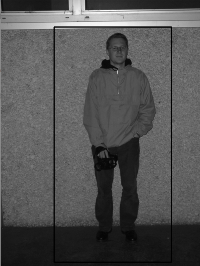
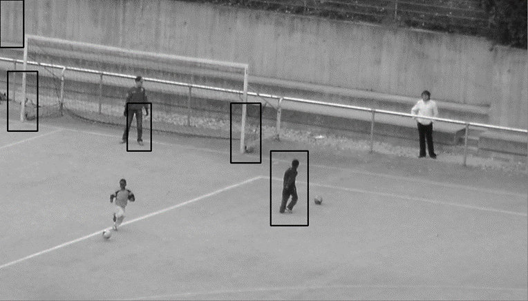
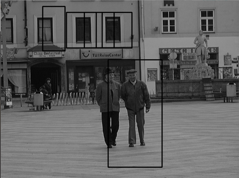
结果只能说是差强人意吧,HOG+SVM模型的上限应该就是这样了。我发现它特别喜欢把一些柱状物体(比如路灯杆、窗框)等识别成人,可能是它们的HOG特征比较相近的缘故。
六、总结
这就是HOG+SVM实现行人检测的全部内容了,我不能保证这种实现方式是最优的,对某些参数进行调整可能使SVM的性能进一步提升,大家在实践的过程中可以自己探索~
参考资料
- https://en.wikipedia.org/wiki/Histogram_of_oriented_gradients
- https://learnopencv.com/histogram-of-oriented-gradients/
- https://courses.cs.duke.edu/fall15/compsci527/notes/hog.pdf
- https://baike.baidu.com/item/HOG/9738560
- https://blog.csdn.net/jingyu_1/article/details/124217455
- Dalal, N., & Triggs, B. (2005). Histograms of oriented gradients for human detection. 2005 IEEE Computer Society Conference on Computer Vision and Pattern Recognition (CVPR’05), 1, 886-893 vol. 1.
- https://zhuanlan.zhihu.com/p/594165143
- https://zhuanlan.zhihu.com/p/27202924
- https://zhuanlan.zhihu.com/p/78504109