常用优化算法(模拟退火、遗传算法、粒子群算法）及其Python实现

模拟退火算法

步骤

Python实现

模拟退火算法

模拟退火算法（Simulated Annealing）是一种全局优化算法，通常用于求解复杂的非凸优化问题。其基本思想是以一定的概率接受劣解，以避免陷入局部最优解，从而在全局范围内搜索最优解。

步骤

模拟退火算法的步骤如下：

在每个降温周期中，接受劣解的概率随着温度的下降而逐渐降低，从而逐渐收敛到全局最优解。不过模拟退火算法的效果和结果很大程度上取决于初始温度、退火速率和终止条件等参数的设置。

Python实现

下面以求解一元函数的全局最小值为例，演示如何使用Python进行模拟退火算法的实现。

首先定义目标函数：

import math
import random
def func(x):
    return x ** 2 + math.sin(5 * x)

只管看一下该函数的样子：

import matplotlib.pyplot as plt
import numpy as np
xarray = np.linspace(-5,5,10000)
plt.plot(xarray,[func(x) for x in xarray])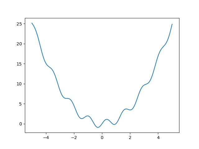

定义模拟退火算法

def simulated_annealing(func, x0, T0, r, iter_max, tol):
    '''
    func 是目标函数
    x0 是初始解
    T0 是初始温度
    r 是退火速率
    iter_max 是最大迭代次数
    tol 是温度下限
    '''
    
    x_best = x0
    f_best = func(x0)
    T = T0
    iter = 0
    while T > tol and iter < iter_max: # 判断是否达到停止条件
        x_new = x_best + random.uniform(-1, 1) * T # 生成新解
        f_new = func(x_new) # 计算目标函数值（适应度值）
        delta_f = f_new - f_best # 能量差
        if delta_f < 0 or random.uniform(0, 1) < math.exp(-delta_f / T): # 决定是否接受
            x_best, f_best = x_new, f_new
        T *= r # 降温 
        iter += 1 # 增加迭代次数
    return x_best, f_best

设置初始参数，求解：

x0 = 2
T0 = 100
r = 0.95
iter_max = 10000
tol = 0.0001
x_best, f_best = simulated_annealing(func, x0, T0, r, iter_max, tol)
print("x_best = {:.4f}, f_best = {:.4f}".format(x_best, f_best))

结果为：x_best = -0.2906, f_best = -0.9086

结果还是比较理想的。

遗传算法

遗传算法是受到生物进化的启发一种优化算法，模拟了生物进化的过程，通过自然选择和遗传操作来逐步优化问题的解。遗传算法是一种常用的优化算法，适用于许多不易解决的实际问题。它有良好的全局搜索能力、强大的适应性和鲁棒性，但也存在一些缺点，如收敛速度较慢、可能陷入局部最优解等。

步骤

遗传算法的基本步骤包括：

初始化种群：根据问题的特性和要求，随机生成一定数量的解，作为初始的种群。
评估适应度：根据问题的评价函数，对每个解进行适应度评估，用于后续的选择和遗传操作。
选择操作：按照适应度大小，选择出一定数量的个体，作为下一代种群的父代。
遗传操作：通过交叉、变异等操作，生成下一代种群的子代。
重复步骤2~4，直到满足停止条件（如达到一定代数、找到最优解等）。

下面以一个简单的实例介绍遗传算法的应用过程。

以函数，我们要求这个函数在区间 [0,15] 上的最大整数值。首先，我们需要初始化种群。设每个个体的基因长度为4（即用4个二进制数表示一个个体，比如0010，表示2），则可以随机生成4个二进制数，如1101、0110、0011，0001等，作为初始的种群。根据这些个体，我们可以通过转换为十进制数，得到对应的函数值。比如，1101 对应的十进制数为 13，代入函数中得到 f(13)=242，这就是个体 1101 的适应度。

接下来，进行选择操作。常用的选择操作有轮盘赌选择、竞争选择等。这里我们使用轮盘赌选择，按照适应度大小将个体分配到轮盘上，再随机选择一定数量的个体作为父代。

然后，进行遗传操作（交叉、变异等）。这里我们使用单点交叉和位变异。假设随机选择个体 1101 和 0011 进行交叉，交叉点为第2位，交叉后得到子代 1111 和 0001。然后，我们对子代进行位变异，即随机选择一位，将其取反。比如 1111 的第3位进行变异，变异后得到子代 1011。

最后，评估适应度，将父代和子代的适应度进行比较。假设子代 1111 和子代 1011 的适应度分别为 f(15)=260 和 f(11)=142。与父代相比，子代中适应度更高的个体将被选择为下一代种群的成员。

重复以上步骤，直到满足停止条件。

Python 实现

import math

def func(x):
    return x**2 + math.sin(5*x)

def fitness(x):
    return 30-(x**2 + math.sin(5*x))
import random

POPULATION_SIZE = 50
GENE_LENGTH = 16

def generate_population(population_size, gene_length):
    population = []
    for i in range(population_size):
        individual = [random.randint(0, 1) for j in range(gene_length)]
        population.append(individual)
    return population

population = generate_population(POPULATION_SIZE, GENE_LENGTH)
def crossover(parent1, parent2):
    crossover_point = random.randint(0, GENE_LENGTH - 1)
    child1 = parent1[:crossover_point] + parent2[crossover_point:]
    child2 = parent2[:crossover_point] + parent1[crossover_point:]
    return child1, child2

def mutation(individual, mutation_probability):
    for i in range(GENE_LENGTH):
        if random.random() < mutation_probability:
            individual[i] = 1 - individual[i]
    return individual

def select_parents(population):
    total_fitness = sum([fitness(decode(individual)) for individual in population])
    parent1 = None
    parent2 = None
    while parent1 == parent2:
        parent1 = select_individual(population, total_fitness)
        parent2 = select_individual(population, total_fitness)
    return parent1, parent2

def select_individual(population, total_fitness):
    r = random.uniform(0, total_fitness)
    fitness_sum = 0
    for individual in population:
        fitness_sum += fitness(decode(individual))
        if fitness_sum > r:
            return individual
    return population[-1]
def decode(individual):
    x = sum([gene*2**i for i, gene in enumerate(individual)])
    return -5 + 10 * x / (2**GENE_LENGTH - 1)

GENERATIONS = 100
CROSSOVER_PROBABILITY = 0.8
MUTATION_PROBABILITY = 0.05

def genetic_algorithm():
    population = generate_population(POPULATION_SIZE, GENE_LENGTH)
    for i in range(GENERATIONS):
        new_population = []
        for j in range(int(POPULATION_SIZE/2)):
            parent1, parent2 = select_parents(population)
            if random.random() < CROSSOVER_PROBABILITY:
                child1, child2 = crossover(parent1, parent2)
            else:
                child1, child2 = parent1, parent2
            child1 = mutation(child1, MUTATION_PROBABILITY)
            child2 = mutation(child2, MUTATION_PROBABILITY)
            new_population.append(child1)
            new_population.append(child2)
        population = new_population
    best_individual = max(population, key=lambda individual: fitness(decode(individual)))
    best_fitness = fitness(decode(best_individual))
    best_x = decode(best_individual)
    best_func = func(best_x)
    return best_x, best_fitness,best_func

best_x, best_fitness,best_func = genetic_algorithm()

print("x = ", best_x)
print("最大适应度为", best_fitness)
print("函数值为",best_func)

注意我在这里将适应度函数fitness设的与函数值不同，是因为我们希望求最小值，而适应度函数在本算法中是越大越好，所以做了微微调整。

粒子群算法

粒子群优化算法

粒子群算法 (Particle Swarm Optimization, PSO) 是一种常用的优化算法，它是一种演化计算技术，源于对鸟群捕食行为的研究。该算法通过模拟鸟群捕食行为中的信息交流和合作，来寻找最优解。具体来说，算法通过在解空间中随机生成一定数量的“粒子”，每个粒子表示一个解，然后通过不断调整每个粒子的位置和速度，使它们向着最优解的方向移动，从而逐步逼近最优解。

步骤

(1)依照初始化过程, 对粒子群的随机位置和速度进行初始设定;
(2)计算每个粒子的适应值;
(3)对于每个粒子, 将其适应值与所经历过的最好位置的适应值进行比较, 若较好, 则将其作为当前最好位置;
(4)对于每个粒子, 将其适应值与全局所经历过的最好位置的适应值进行比较, 若较好, 则将其作为当前的全局最好位置;
(5)根据两个迭代公式对粒子的速度和位置进行进化;
(6)如末达到结束条件通常为足够好的适应值或达到一个预设最大代数(Gmax), 返回步骤(2); 否则执行步骤 (7)
(7)输出gbest.

Python实现

还是求函数在[-5,5]上的最小值

import numpy as np

def evaluate_fitness(x):
    return x ** 2 + np.sin(5*x)

class PSO:
    def __init__(self, n_particles, n_iterations, w, c1, c2, bounds):
        self.n_particles = n_particles
        self.n_iterations = n_iterations
        self.w = w
        self.c1 = c1
        self.c2 = c2
        self.bounds = bounds

        self.particles_x = np.random.uniform(bounds[0], bounds[1], size=(n_particles,))
        self.particles_v = np.zeros_like(self.particles_x)
        self.particles_fitness = evaluate_fitness(self.particles_x)
        self.particles_best_x = self.particles_x.copy()
        self.particles_best_fitness = self.particles_fitness.copy()

        self.global_best_x = self.particles_x[self.particles_fitness.argmin()]

    def update_particle_velocity(self):
        r1 = np.random.uniform(size=self.n_particles)
        r2 = np.random.uniform(size=self.n_particles)

        self.particles_v = self.w * self.particles_v + \
            self.c1 * r1 * (self.particles_best_x - self.particles_x) + \
            self.c2 * r2 * (self.global_best_x - self.particles_x)

        self.particles_v = np.clip(self.particles_v, -1, 1)

    def update_particle_position(self):
        self.particles_x = self.particles_x + self.particles_v

        self.particles_x = np.clip(self.particles_x, self.bounds[0], self.bounds[1])

        self.particles_fitness = evaluate_fitness(self.particles_x)

        better_mask = self.particles_fitness < self.particles_best_fitness
        self.particles_best_x[better_mask] = self.particles_x[better_mask]
        self.particles_best_fitness[better_mask] = self.particles_fitness[better_mask]

        best_particle = self.particles_fitness.argmin()
        if self.particles_fitness[best_particle] < evaluate_fitness(self.global_best_x):
            self.global_best_x = self.particles_x[best_particle]

    def run(self):
        for i in range(self.n_iterations):
            self.update_particle_velocity()
            self.update_particle_position()

            #print("Iteration:", i, "Global Best:", self.global_best_x)

        return self.global_best_x

pso = PSO(n_particles=20, n_iterations=50, w=0.7, c1=1.4, c2=1.4, bounds=(-5, 5))
global_best_x = pso.run()

上述代码中，首先定义了一个 evaluate_fitness 函数来计算适应度值,其实就是函数值。然后，定义了一个 PSO 类来实现粒子群算法。在初始化过程中，随机生成了一定数量的粒子，并计算它们的适应度值。然后，在每次迭代中，分别更新每个粒子的速度和位置，并更新每个粒子的最优位置和全局最优位置。最后，我们输出最终的全局最优位置。

最优解为：-0.290836630206147。