图像识别流程学习总结

通过图像识别的学习，初步总结了图像识别的流程及归类，希望可以帮到正在学习的小伙伴。
在这里插入图片描述
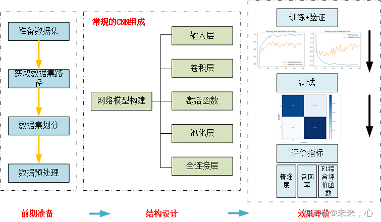
一、前期准备工作
1、数据集的获取
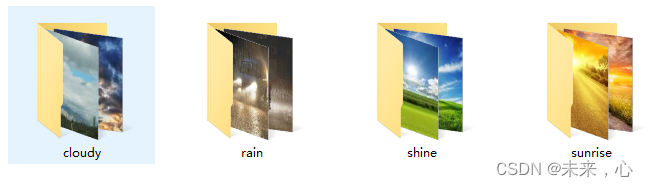
在进行数据分析之前需要有数据进行识别，这里所谓的数据指的是图像，我们需要对需要识别的图像分好其类别才能更好的调用。下面以天气数据集为例，共分为四类，数据集划分如下图所示：

['cloudy', 'rain', 'shine', 'sunrise']

在这里插入图片描述
2、获取数据集路径
获取数据集的方法有很多，这里使用的是pathlib函数库，也可以使用os函数库获取数据

import pathlib
data_dir = "G:\BaiduNetdiskDownload\climate\weather_photos/"
data_dir = pathlib.Path(data_dir)
#查看数据数量
image_count = len(list(data_dir.glob('*/*.jpg')))

3、数据集划分
这里函数validation_split将数据集划分为0.8:0.2即4:1

#训练集
train_ds = tf.keras.preprocessing.image_dataset_from_directory(
    data_dir,
    validation_split=0.2,
    subset="training",
    seed=123,
    image_size=(img_height, img_width),
    batch_size=batch_size)
#验证集
val_ds = tf.keras.preprocessing.image_dataset_from_directory(
    data_dir,
    validation_split=0.2,
    subset="validation",
    seed=123,
    image_size=(img_height, img_width),
    batch_size=batch_size)

4、数据预处理

shuffle():打乱数据，关于此函数的详细介绍可以参考: https:lzhuanlan.zhihu.com/p/42417456
prefetch():预取数据，加速运行
在这里插入图片描述

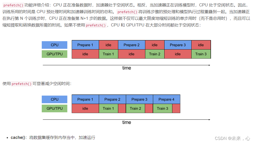
AUTOTUNE = tf.data.AUTOTUNE
train_ds = train_ds.cache().shuffle(1000).prefetch(buffer_size=AUTOTUNE)
val_ds = val_ds.cache().prefetch(buffer_size=AUTOTUNE)
num_classes = 4
batch_size = 32
img_height = 180
img_width = 180

二、网络模型构建
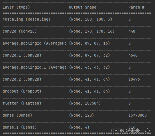
1、模型搭建
卷积神经网络的基本组成包括输入层、卷积层、激活函数、池化层、全连接层（放在最后作为输出层）等组成。各层的主要功能这里不在详细介绍，可以参考连接
直接上代码：

model = models.Sequential([
    layers.experimental.preprocessing.Rescaling(1. / 255, input_shape=(img_height, img_width, 3)),

    layers.Conv2D(16, (3, 3), activation='relu', input_shape=(img_height, img_width, 3)),  # 卷积层1，卷积核3*3
    layers.AveragePooling2D((2, 2)),  # 池化层1，2*2采样
    layers.Conv2D(32, (3, 3), activation='relu'),  # 卷积层2，卷积核3*3
    layers.AveragePooling2D((2, 2)),  # 池化层2，2*2采样
    layers.Conv2D(64, (3, 3), activation='relu'),  # 卷积层3，卷积核3*3
    layers.Dropout(0.3),

    layers.Flatten(),  # Flatten层，连接卷积层与全连接层
    layers.Dense(128, activation='relu'),  # 全连接层，特征进一步提取
    layers.Dense(num_classes)  # 输出层，输出预期结果
])

model.summary()  # 打印网络结构

其网络详细参数可通过**model.summary()**打印出
在这里插入图片描述
2、网络配置
包括优化器的选取、算是函数的选取、学习率的设计

# 编译 设置优化器
#learning_rate=0.001学习率
opt = tf.keras.optimizers.Adam(learning_rate=0.001)

model.compile(optimizer=opt,
              loss=tf.keras.losses.SparseCategoricalCrossentropy(from_logits=True),
              metrics=['accuracy'])

三、模型评价
1、训练+验证

epochs = 50#训练次数

history = model.fit(
  train_ds,
  validation_data=val_ds,
  epochs=epochs
)

训练过程可视化代码

acc = history.history['accuracy']
val_acc = history.history['val_accuracy']

loss = history.history['loss']
val_loss = history.history['val_loss']

epochs_range = range(epochs)

plt.figure(figsize=(12, 4))
plt.subplot(1, 2, 1)
plt.plot(epochs_range, acc, label='Training Accuracy')
plt.plot(epochs_range, val_acc, label='Validation Accuracy')
plt.legend(loc='lower right')
plt.title('Training and Validation Accuracy')

plt.subplot(1, 2, 2)
plt.plot(epochs_range, loss, label='Training Loss')
plt.plot(epochs_range, val_loss, label='Validation Loss')
plt.legend(loc='upper right')
plt.title('Training and Validation Loss')
plt.show()

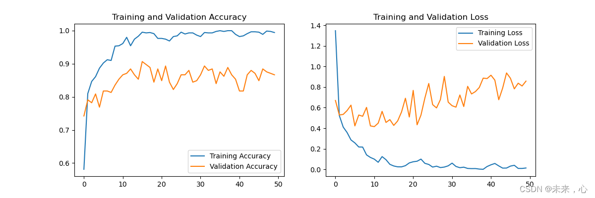
训练过程如下图
在这里插入图片描述
2、评价
将训练的模型进行保存，用于评价预测结果时调用

model.save('./checkpoint/model.h5')
#评价结果
score = model.evaluate_generator(Generator(testpath,batch_size),steps=int(m) // batch_size)

评价公式如下

def Precision(y_true, y_pred):
    """精确率"""
    tp = K.sum(K.round(K.clip(y_true * y_pred, 0, 1)))  # true positives
    pp = K.sum(K.round(K.clip(y_pred, 0, 1)))  # predicted positives
    precision = tp / (pp + K.epsilon())
    return precision

def Recall(y_true, y_pred):
    """召回率"""
    tp = K.sum(K.round(K.clip(y_true * y_pred, 0, 1)))  # true positives
    pp = K.sum(K.round(K.clip(y_true, 0, 1)))  # possible positives
    recall = tp / (pp + K.epsilon())
    return recall


def F1(y_true, y_pred):
    """F1-score"""
    precision = Precision(y_true, y_pred)
    recall = Recall(y_true, y_pred)
    f1 = 2 * ((precision * recall) / (precision + recall + K.epsilon()))
    return f1

如何使用，请参考链接

图像识别流程学习总结

猜你喜欢