课后作业

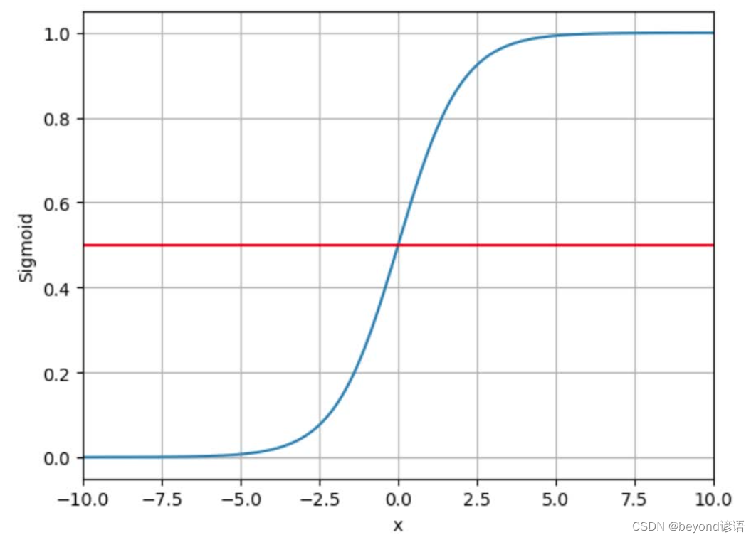
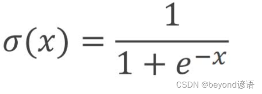
①Logistic函数

sigmoid函数是一类非线性激活函数的统称，但因为Logistic使用人数多且高效，故进而将sigmoid函数等价于Logistic函数。

Logistic图形和具体公式如下：
在这里插入图片描述

②回归和分类

我个人觉得：
回归问题就是输入个x，输出一个对应的y，且y∈R
例如y = 2 * x，给定一个x，就会得到一个y

分类问题就是给定一个x，输出具体的y，也就是几个类别，是1还是0
例如超过60分表示及格，输入一个x，x为90，输出结果为1，表示及格；x为40，y为0，表示不及格

原理大概就是这样，如何实现，就需要使用激活函数了，以Logistic Function为例，这个函数可以将任意一个输入x∈R，输出结果映射到[0,1]之间，这样就变成了概率问题
例如二分类问题，输入x，输出结果为1的概率是0.8，结果为0的概率是0.2，那么这个x就属于1这个类别

tensor数据类型包括data和grad，data存放数据，常使用.item()来获取具体的数值，这样占用内存较小；grad存放梯度，但需要提前对tensor对象通过.requires_grad进行设置为True

③模型架构

这是一个大体通用的模型架构
LinearModel类名可自定义，但必须继承torch.nn.Module
内部的两个函数__init__和forward必须有，且不可以改写函数名，这是在继承的父类里面进行模块重写
super(LinearModel,self).__init__()必须对指定的父类初始化，其中LinearModel跟自己定义的类名一致
torch.nn.Linear(1,1)线性层，输入维度和输出维度都是1维
__init__函数中为了初始化
forward函数为了前向传播计算梯度
因为sigmoid函数在torch.nn.functional包内，故需要导包
F.sigmoid(self.linear(x))对经过一层线性层得出的结果通过sigmoid函数映射到[0,1]内，方便进行概率的计算，以至于最终的分类

import torch.nn.functional as F

class LinearModel(torch.nn.Module):
    def __init__(self):
        super(LinearModel,self).__init__()
        self.linear = torch.nn.Linear(1,1)
    
    
    def forward(self,x):
        y_hat = F.sigmoid(self.linear(x))
        return y_hat

④代码实现

需求：分类任务
x≤2时，y=0，属于0类
x＞2时，y=1，属于1类
训练样本：x=1，y=0；x=2，y=0；x=3，y=1
损失函数使用BCELoss，交叉熵损失函数；细节等详细信息可参考该篇博文：六、逻辑回归
优化器使用SGD
进行10000次epoch

import torch
import torch.nn.functional as F
import matplotlib.pyplot as plt

x_data = torch.Tensor([[1.],[2.],[3.]])
y_data = torch.Tensor([[0],[0],[1]])

class LinearModel(torch.nn.Module):
    def __init__(self):
        super(LinearModel,self).__init__()
        self.linear = torch.nn.Linear(1,1)
    
    
    def forward(self,x):
        y_hat = F.sigmoid(self.linear(x))
        return y_hat

model = LinearModel()


lossf = torch.nn.BCELoss(size_average=False)            #损失函数
optimzer = torch.optim.SGD(model.parameters(),lr=0.001)  #优化器

loss_all = []  #把每次训练的损失都存下来，方便后续绘图看效果
epoch_all = [] #每次的epoch存下来，方便绘图

for epoch in range(10000):
    y_pred = model(x_data)
    loss = lossf(y_pred,y_data)
    print("epoch:",epoch,"\tloss:",loss.item())
    epoch_all.append(epoch)
    loss_all.append(loss)
    optimzer.zero_grad()
    loss.backward()
    optimzer.step()

# 绘图
plt.plot(loss_all,epoch_all)
plt.ylabel('loss Value')
plt.xlabel('Epoch')
plt.show()

在这里插入图片描述
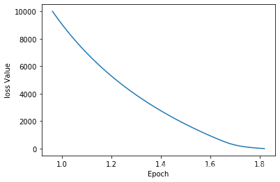
还得多epoch几次，loss没降下去，先就这样了，学会方法就行，效果后期再考虑

⑤测试模型

test = torch.Tensor([[4.]]) # 用4去测试一下
resutl = model(test)
if resutl.item()>0.5:
    print("1")
else:
    print("0")

print("predect value is:",model(test).item()) #看下预测x=4时，y的值是多少
"""
1
predect value is: 0.8959792256355286
"""

结果对了，x＞2时，y=1，属于1类

五、Logistic Function