In this document the first 4 steps of the JPEG encoding chain are demonstrated. These 4 steps contain the lossy parts of the coding. The remaining steps, i.e. runlength and Huffman encoding, are losless. Therefore the 4 steps demonstrated here are sufficient to study the quality-loss of JPEG encoding.
在本文档中,演示了JPEG编码链的前4个步骤。这4个步骤包含了编码的有损部分。剩下的步骤,即runlength和Huffman编码,是无损的。因此,本文的4个步骤足以研究JPEG编码的质量损失。
The following packages are required.:
需要准备以下软件包:
import cv2
import numpy as np
from matplotlib import pyplot as plt
import matplotlib.cm as cm
Step 1: Read and display image
步骤1:读取和显示图像
In OpenCV color images are imported as BGR. In order to display the image with pyplot.imshow() the channels must be switched such that the order is RGB.:
在OpenCV中,彩色图像作为BGR导入。为了使用pyplot.imshow()显示图像,通道必须切换为RGB顺序。
B=8 # blocksize (In Jpeg the
img1 = cv2.imread("lichtenstein.png", cv2.CV_LOAD_IMAGE_UNCHANGED)
h,w=np.array(img1.shape[:2])/B * B
img1=img1[:h,:w]
#Convert BGR to RGB
img2=np.zeros(img1.shape,np.uint8)
img2[:,:,0]=img1[:,:,2]
img2[:,:,1]=img1[:,:,1]
img2[:,:,2]=img1[:,:,0]
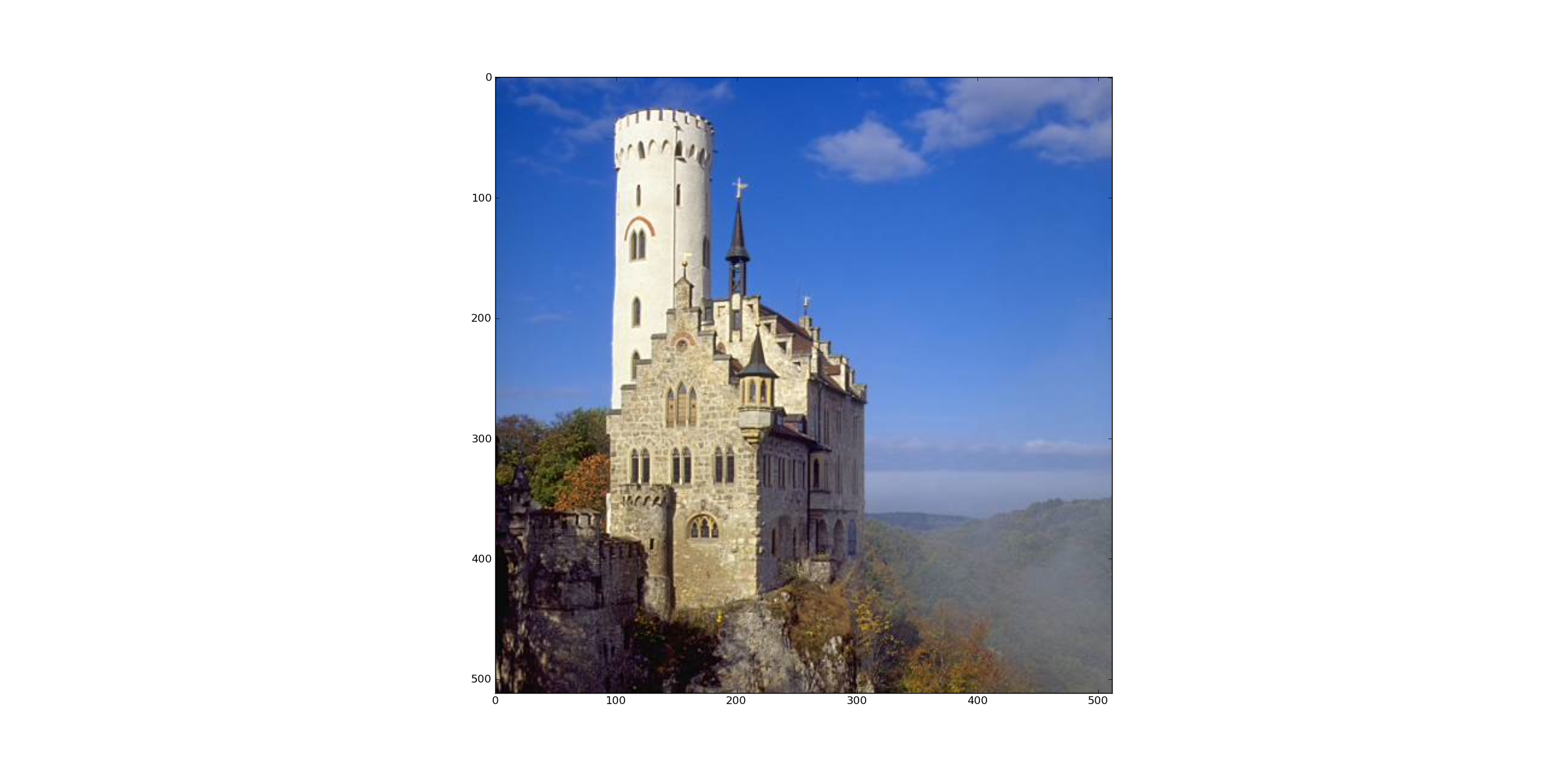
plt.imshow(img2)The user is asked to click into the image. The clicked block is highlighted in the image (blue rectangle). For the clicked block the DCT coefficients will be displayed later:
用户被要求点击图像。单击的块在图像中突出显示(蓝色矩形)。对于被点击的方块,DCT系数稍后会显示:
point=plt.ginput(1)
block=np.floor(np.array(point)/B) #first component is col, second component is row
print "Coordinates of selected block: ",block
scol=block[0,0]
srow=block[0,1]
plt.plot([B*scol,B*scol+B,B*scol+B,B*scol,B*scol],[B*srow,B*srow,B*srow+B,B*srow+B,B*srow])
plt.axis([0,w,h,0])
Step 2: Transform BGR to YCrCb and Subsample Chrominance Channels
步骤2:将BGR转换为YCrCb和子样本色度通道
Using OpenCV the color space transform is implemented by:
使用OpenCV实现颜色空间变换:
transcol=cv2.cvtColor(img1, cv2.cv.CV_BGR2YCrCb)Next, the chrominance channels Cr and Cb are subsampled. The constant SSH defines the subsampling factor in horicontal direction, SSV defines the vertical subsampling factor. Before subsampling the chrominance channels are filtered using a (2x2) box filter (=average filter). After subsampling all 3 channels are stored in the list imSub:
其次,对色度通道Cr和Cb进行下采样。常数SSH定义水平方向的子采样因子,SSV定义垂直方向的子采样因子。在子采样之前,使用(2x2)盒形滤波器(=平均滤波器)对色度通道进行滤波。子采样后,所有3个通道存储在列表imSub:
SSV=2
SSH=2
crf=cv2.boxFilter(transcol[:,:,1],ddepth=-1,ksize=(2,2))
cbf=cv2.boxFilter(transcol[:,:,2],ddepth=-1,ksize=(2,2))
crsub=crf[::SSV,::SSH]
cbsub=cbf[::SSV,::SSH]
imSub=[transcol[:,:,0],crsub,cbsub]
Step 3 and 4: Discrete Cosinus Transform and Quantisation
步骤3和4:离散余弦变换和量化
First the quantisation matrices for the luminace channel (QY) and the chrominance channels (QC) are defined, as proposed in the annex of the Jpeg standard.:
首先定义了亮度通道(QY)和色度通道(QC)的量化矩阵,如Jpeg标准附件中所述:
QY=np.array([[16,11,10,16,24,40,51,61],
                         [12,12,14,19,26,48,60,55],
                         [14,13,16,24,40,57,69,56],
                         [14,17,22,29,51,87,80,62],
                         [18,22,37,56,68,109,103,77],
                         [24,35,55,64,81,104,113,92],
                         [49,64,78,87,103,121,120,101],
                         [72,92,95,98,112,100,103,99]])

QC=np.array([[17,18,24,47,99,99,99,99],
                         [18,21,26,66,99,99,99,99],
                         [24,26,56,99,99,99,99,99],
                         [47,66,99,99,99,99,99,99],
                         [99,99,99,99,99,99,99,99],
                         [99,99,99,99,99,99,99,99],
                         [99,99,99,99,99,99,99,99],
                         [99,99,99,99,99,99,99,99]])
In order to provide different quality levels a quality factor QF can be selected. From the quality factor the scale parameter is calculated. The matrices defined above are multiplied by the scale parameter. A low quality factor implies are large scale parameter. A large scale parameter yields a coarse quantisation, a low quality but a high compression rate. The list Q contains the 3 scaled quantisation matrices, which will be applied to the DCT coefficients:
为了提供不同的质量水平,可以选择质量因子QF。由质量因子计算尺度参数。上面定义的矩阵乘以scale参数。低质量因子意味着大尺度参数。一个大尺度的参数产生一个粗糙的量化,一个低质量但高压缩率。列表Q包含3个缩放量化矩阵,将其应用于DCT系数:
QF=99.0
if QF < 50 and QF > 1:
        scale = np.floor(5000/QF)
elif QF < 100:
        scale = 200-2*QF
else:
        print "Quality Factor must be in the range [1..99]"
scale=scale/100.0
Q=[QY*scale,QC*scale,QC*scale]
In the following loop DCT and quantisation is performed channel by channel. As defined in the standard, before DCT the pixel values of all channels are shifted by -128, such that the new value range is [-128,...127]. The loop iterates over the imSub-list, which contains the 3 channels. The result of the DCTs of the 3 channels are stored in 2-dimensional numpy arrays, which are put into the python list TransAll. Similarly the quantized DCT coefficients are stored in 2-dimensional numpy arrays, which are assigned to the python list TransAllQuant. Note that the channels have different shapes due to chrominance subsampling. In the last part of the loop the DCT coefficients of the previously selected and highlighted block are displayed:
在接下来的环路中,DCT和量化是一个通道接着一个通道地执行。如标准中定义的,在DCT之前,所有通道的像素值都要偏移-128,使得新的取值范围为[-128,…127]。循环遍历imsub列表,其中包含3个通道。3个通道的dct的结果存储在二维numpy数组中,这些数组被放入python列表TransAll中。类似地,量化的DCT系数存储在二维numpy数组中,这些数组被分配给python列表TransAllQuant。注意,通道有不同的形状
TransAll=[]
TransAllQuant=[]
ch=['Y','Cr','Cb']
plt.figure()
for idx,channel in enumerate(imSub):
        plt.subplot(1,3,idx+1)
        channelrows=channel.shape[0]
        channelcols=channel.shape[1]
        Trans = np.zeros((channelrows,channelcols), np.float32)
        TransQuant = np.zeros((channelrows,channelcols), np.float32)
        blocksV=channelrows/B
        blocksH=channelcols/B
        vis0 = np.zeros((channelrows,channelcols), np.float32)
        vis0[:channelrows, :channelcols] = channel
        vis0=vis0-128
        for row in range(blocksV):
                for col in range(blocksH):
                        currentblock = cv2.dct(vis0[row*B:(row+1)*B,col*B:(col+1)*B])
                        Trans[row*B:(row+1)*B,col*B:(col+1)*B]=currentblock
                        TransQuant[row*B:(row+1)*B,col*B:(col+1)*B]=np.round(currentblock/Q[idx])
        TransAll.append(Trans)
        TransAllQuant.append(TransQuant)
        if idx==0:
                selectedTrans=Trans[srow*B:(srow+1)*B,scol*B:(scol+1)*B]
        else:
                sr=np.floor(srow/SSV)
                sc=np.floor(scol/SSV)
                selectedTrans=Trans[sr*B:(sr+1)*B,sc*B:(sc+1)*B]
        plt.imshow(selectedTrans,cmap=cm.jet,interpolation='nearest')
        plt.colorbar(shrink=0.5)
        plt.title('DCT of '+ch[idx])
Decoding
解码
In order to show the quality decrease caused by the Jpeg coding the 4 steps performed above are inverted in order to decode the image. In the following loop for each channel first the inverse quantisation is performed, followed by the inverse dct and the inverse shiftign of the shift of the pixel values, sucht that their value range is [0,...,255]. Moreover the subsampled chrominance channels are interpolated, using the opencv method resize() such that their original size is reconstructed.:
为了显示Jpeg编码造成的质量下降,将上述4步进行倒排,以解码图像。在接下来的循环中,对每个通道首先执行逆量化,然后是逆dct和像素值的移位的逆移位,这样它们的值范围是[0,…,255]。此外,使用opencv方法resize()对下采样的色度信道进行插值,从而重构其原始大小。
DecAll=np.zeros((h,w,3), np.uint8)
for idx,channel in enumerate(TransAllQuant):
        channelrows=channel.shape[0]
        channelcols=channel.shape[1]
        blocksV=channelrows/B
        blocksH=channelcols/B
        back0 = np.zeros((channelrows,channelcols), np.uint8)
        for row in range(blocksV):
                for col in range(blocksH):
                        dequantblock=channel[row*B:(row+1)*B,col*B:(col+1)*B]*Q[idx]
                        currentblock = np.round(cv2.idct(dequantblock))+128
                        currentblock[currentblock>255]=255
                        currentblock[currentblock<0]=0
                        back0[row*B:(row+1)*B,col*B:(col+1)*B]=currentblock
        back1=cv2.resize(back0,(h,w))
        DecAll[:,:,idx]=np.round(back1)
The 3-dimensional numpy-array DecAll contains the decoded YCrCb image. This image is backtransformed to BGR, stored to a file and displayed in a pyplot figure. Finally the Sum of squared error (SSE) between the original image and the decoded image is calculated:
三维数字数组DecAll包含解码后的YCrCb图像。此图像被反转换为BGR,存储到一个文件并在pyplot图中显示。最后计算原始图像与解码图像之间的平方误差之和(Sum of squared error, SSE):
reImg=cv2.cvtColor(DecAll, cv2.cv.CV_YCrCb2BGR)
cv2.cv.SaveImage('BackTransformedQuant.jpg', cv2.cv.fromarray(reImg))
plt.figure()
img3=np.zeros(img1.shape,np.uint8)
img3[:,:,0]=reImg[:,:,2]
img3[:,:,1]=reImg[:,:,1]
img3[:,:,2]=reImg[:,:,0]
plt.imshow(img3)
SSE=np.sqrt(np.sum((img2-img3)**2))
print "Sum of squared error: ",SSE
plt.show()
The SSE for different quality factors and subsampling schemes is displayed in the table below.
不同质量因素和子抽样方案的SSE如下表所示。
| Subsampling | Quality Factor | SSE |
| 4:2:0 | 10 | 6330 |
| 4:2:0 | 40 | 4740 |
| 4:2:0 | 70 | 4170 |
| 4:2:0 | 99 | 2545 |
| 4:4:4 | 99 | 1885 |
The following images demonstrate the quality decrease with decreasing quality factor QF.
以下图像显示质量随着质量因子QF的下降而下降。

Subsampling 4:2:0, Quality Factor QF=10

Subsampling 4:2:0, Quality Factor QF=40
Subsampling 4:2:0, Quality Factor QF=70