1 Abstract 解读
摘要中主要介绍了它相对于之前网络上性能的提升:
At 320 × 320 YOLOv3 runs in 22 ms at 28.2 mAP,as accurate as SSD but three times faster.
yolov3在输入图片为 320 × 320 的大小下,处理时间为 22ms,换算下来大概 50FPS,并且在COCO数据集上达到了 28.2mAP 的平均精度,在同样精度下,速度比SSD块了三倍
When we look at the old .5 IOU mAP detection metric YOLOv3 is quite good. It achieves 57.9 AP50 in 51 ms on a Titan X, compared to 57.5 AP50 in 198 ms by RetinaNet, similar performance but 3.8× faster.
这段话说明了,在 0.5 IOU mAP(0.5IOU下的 mAP)的情况下,YOLOv3 的表现也非常出色,它在 Titan X 显卡上,实现 57.9 AP50(在 0.5 IOU 下AP达到了 57.9),每张图片的处理速度是 51 ms,在性能和RetinaNet相似的情况的情况下快了3.8倍。
- IOU的值越大,和真正的预测结果越接近,IOU越小则越偏离。一般有 0.5,0。55,…,0.95,这里的0.5是最低值。(这里就不详细讲解了)
这张图片是目标检测中经常遇到的,我们就来分析一下如何解读这张图片
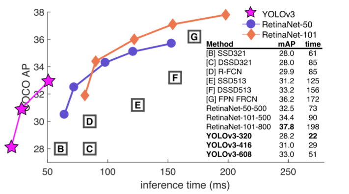
- 这张图片是用来三个网络作对比:YOLOv3、RetinaNet(backbone 为 ResNet 50)、RetinaNet(backbone 为 ResNet 100)
- 从横纵坐标来看:COCO AP 肯定越高越好,inference time(每张图片的推理时间)肯定越小越好
- 注意:这里是以 mAP 作为评价指标,论文后面的图片是以 mAP-50 作为评价指标,mAP 是 mAP-50,mAP-55,…,mAP-95的平均值,mAP-50 只是 mAP 的其中一种情况,因此 mAP-50 下的结果一般比 mAP 高。
2 The Deal 解读
2.1 Bounding Box Prediction
Following YOLO9000 our system predicts bounding boxes using dimension clusters as anchor boxes.
这里说明了YOLOv3还是沿用了YOLO9000(YOLOv2),使用聚类算法来生成 anchor boxes。
The network predicts 4 coordinates for each bounding box, tx,ty, tw, th. If the cell is offset from the top left corner of the image by (cx, cy) and the bounding box prior has width and height pw, ph, then the predictions correspond to:
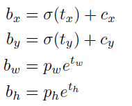
这里说明了YOLO网络会为每个 bounding box(bounding box指的是每个网格对应的 anchor box) 生成四个值 tx,ty, tw, th,其中 tx,ty 作用于 (cx, cy) ,即网格的左上角,tw, th作用于anchor box 的宽高 pw, ph。
经过计算后 bx,by即为物体预测的中心,bw,bh即为anchor box 调整后的宽高。这里说明一下,如果bw,bh如果超过图片的边界,那么就直接算作图片的边界,不管超出的部分。
During training we use sum of squared error loss.
训练时使用 squared error loss。
YOLOv3 predicts an objectness score for each bounding box using logistic regression. This should be 1 if the bounding box prior overlaps a ground truth object by more than any other bounding box prior.If the bounding box prior is not the best but does overlap a ground truth object bymore than some threshold we ignore the prediction.
这里说明了YOLOv3网络针对每个 bounding box 会预测一个 objectness score。如果一个bounding box 和 ground truth 的重叠面积比其它 bounding box 都大,那么这个 bounding box 的 objectness score 就设置为 1。如果一个bounding box 和 ground truth 的重叠面积并不是最大的,但是也超过的某个阈值,我们就 忽略它(也就是进行loss计算的时候不考虑它)。
2.2 Class Prediction
Each box predicts the classes the bounding box may contain using multilabel classification. We do not use a softmax as we have found it is unnecessary for good performance,instead we simply use independent logistic classifiers. During training we use binary cross-entropy loss for the class predictions.
这里说明了网络针对每个 bounding box 会使用多标签分类来预测边界框可能包含的类别。这里没有使用softmax 激活函数,至于为什么在下一段作者有说明。在训练期间,我们使用二元交叉熵损失进行类预测。
This formulation helps when we move to more complex domains like the Open Images Dataset [7]. In this dataset there are many overlapping labels (i.e. Woman and Person). Using a softmax imposes the assumption that each box has exactly one class which is often not the case. A multilabel approach better models the data.
这里说明了在数据集中每个要检测的物体可能会有有多个标签(比如:女人和人)。softmax函数式只有一个输出,即假设每个要检测的目标只有一个标签,这和实际情况明显不符。因此针对一个目标可能有多个标签的情况作者选择了使用 sigmod函数。
2.3 Predictions Across Scales
YOLOv3 predicts boxes at 3 different scales. Our system extracts features from those scales using a similar concept to feature pyramid networks [8]. From our base feature extractor we add several convolutional layers. The last of these predicts a 3-d tensor encoding bounding box, objectness, and class predictions. In our experiments with COCO [10] we predict 3 boxes at each scale so the tensor is N×N× [3 ∗ (4 + 1 + 80)] for the 4 bounding box offsets,1 objectness prediction, and 80 class predictions.
这里说明了YOLOv3会在3种不同的尺度上生成先验框,这个思路来自feature pyramid networks [8]。与feature pyramid networks [8]不同的是YOLOv3还添加了几个卷积层。YOLOv3在每个scale上都会预测3个bounding box,即 N × N × [ 3 × (4 + 1 + 80) ],它的意思是将图片分为 N × N 的网格,每个网格对应 3个 bounding box(预测框),每个预测框有 (4 + 1 + 80) 个参数,4指用于表示边界框偏移的四个参数,1指的是 objectness score,80指的是数据集有多少个类别,比如COCO是80个种类,因此这里是80。
Next we take the feature map from 2 layers previous and upsample it by 2×. We also take a feature map from earlier in the network and merge it with our upsampled features using concatenation. This method allows us to get more meaningful semantic information from the upsampled features and finer-grained information from the earlier feature map. We then add a few more convolutional layers to process this combined feature map, and eventually predict a similar tensor, although now twice the size.
这里说明的是YOLOv3网络中特征融合是怎么做的,首先对本层的 feature map 进行2倍的上采样,然后会将早期网络的 feature map 和上采样之后的 features 进行 拼接(concatenation)。上采样操作能获得更有意义的 语义信息,而早期网络的 feature map 更具有细粒度的信息,将二者融合能更好的识别出我们要检测的目标。然后添加几个卷积层来处理这个拼接后的feature map。
We still use k-means clustering to determine our bounding box priors. We just sort of chose 9 clusters and 3 scales arbitrarily and then divide up the clusters evenly across scales. On the COCO dataset the 9 clusters were:(10×13), (16×30), (33×23), (30×61), (62×45), (59×119), (116 × 90), (156 × 198), (373 × 326).
这里说明了YOLOv3仍然使用 k-means 聚类算法来确定先验框。 任意选择 9 个集群和 3 个尺度,然后在尺度上均匀地划分集群。 在 COCO 数据集上,9 个簇分别为:(10×13)、(16×30)、(33×23)、(30×61)、(62×45)、(59×119)、(116×90) , (156 × 198), (373 × 326)。
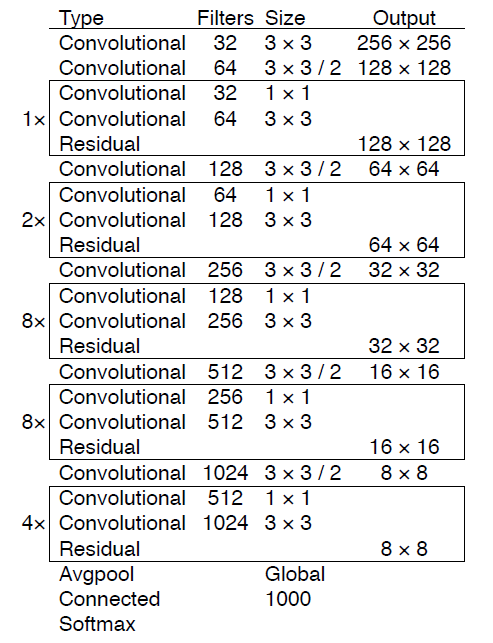
2.4 Feature Extractor(特征提取网络)
YOLOv3使用的是Dartnet-53作为backbone,YOLOv2使用的是Dartnet-19作为backbone,这里就不多介绍了。
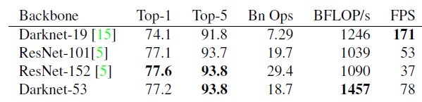
Darknet-53 is better than ResNet-101 and 1.5× faster. Darknet-53 has similar performance to ResNet-152 and is 2× faster.
2.5 Training
We still train on full images with no hard negative mining or any of that stuff. We use multi-scale training, lots of data augmentation, batch normalization, all the standard stuff.We use the Darknet neural network framework for training and testing [14].
这里说明了YOLOv3没有使用困难样本挖掘(小样本、特征不清晰的样本、颜色非常接近的样本等都是困难样本)。使用了 data augmentation、batch normalization等。
3 总结
训练策略
- 对于预测框我们把它分为:正例(positive)、负例(negat ive)、忽略样例(ignore)
- 先验框数量:
- 针对416输入:有10647个bounding boxes
- 针对256输入:有4032个bounding boxes
- 正例:取一个ground truth,与10647个框全部计算IOU,
最大的为正例。正例产生置信度loss、检测框loss、类别loss。 ground truth box为对应的预测框的标签。 - 负例:与全部ground truth的IOU都小于阈值(0.5),则为负例。负例
只有分类置信度产生loss,分类标签为0,边框回归不产生loss。 - 忽略样例:正例除外,与任意一个ground truth的IOU大于阈值(论文中使用0.5),则为忽略样例。
忽略样例不产生任何loss。
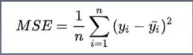
损失函数
- x、y、w、h使用MSE作为损失函数,也可以使用smooth L1 loss
- 分类loss、置信度loss都使用二元交叉损失熵作为loss function
- 对于输入,先进行sigmod处理
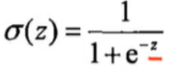
- 然后求BCELoss
