1. Create a relational connection to an Excel spreadsheet or text file using ODBC drivers

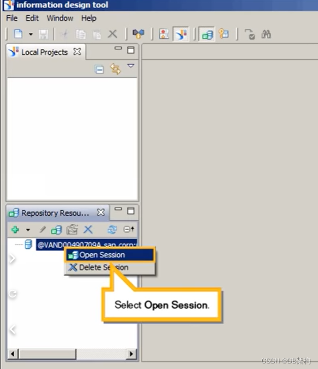
1.1 Select Open Session
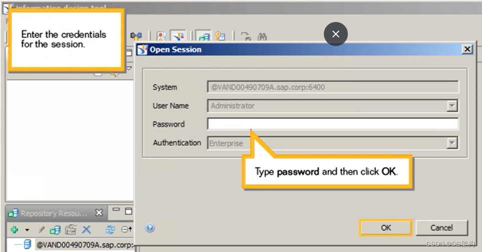
1.2 Enter the credentials for the session.Type password and then click OK.
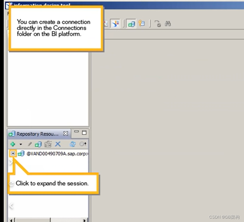
1.3 You can create a connection directly in the Connections folder on the BI platform. click the expend the session.
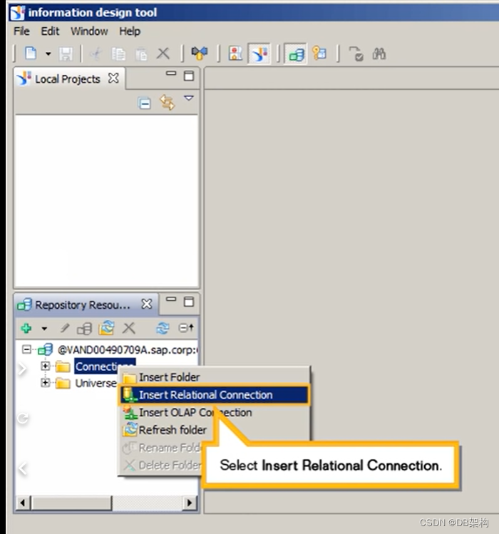
1.4 Right Click the connection folder

1.5 Selection Insert Relational Connection.
1.6 Define a unqiue name for the connection . Type Warehouse_csv and then click the Next >.

1.7 Choose the appropriate driver based on the data source. Click to expand the Microsoft drivers.

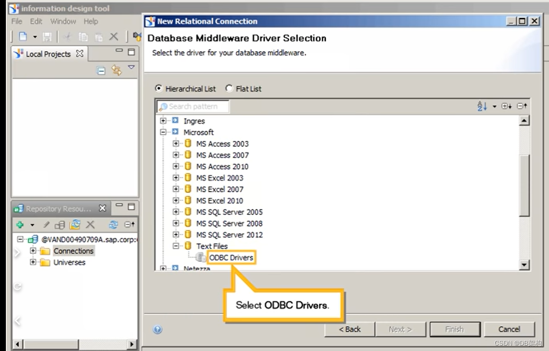
1.8 Choose the driver for the appropriate version of Microsoft Excel for a spreadsheet. or use the Text Files option for a CSV or text file.Click to expand the Text Files data source.

1.9 Select ODBC Drivers.
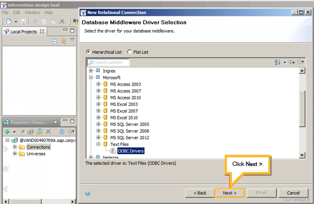
1.10 Click Next>.
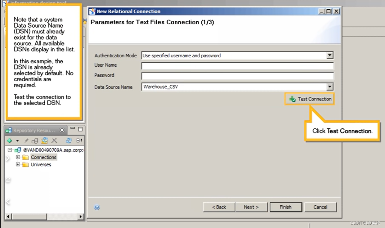
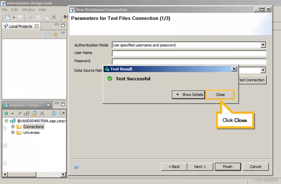
1.11Note that a system Data Source Name (DSN) must already exist for the data source. All avaliable DSNs display in the list. Click Test Connection.
1.12 Click Close.
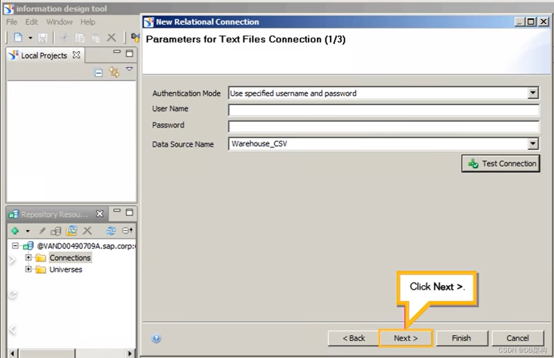
1.13 Click Next>.
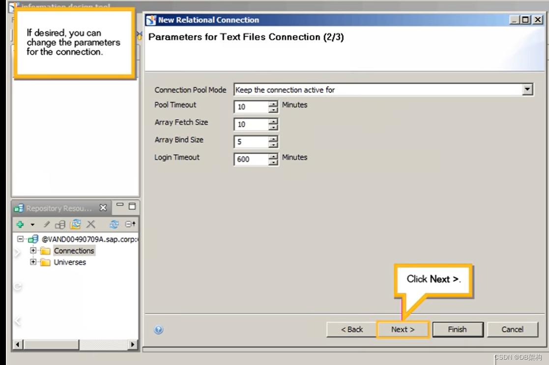
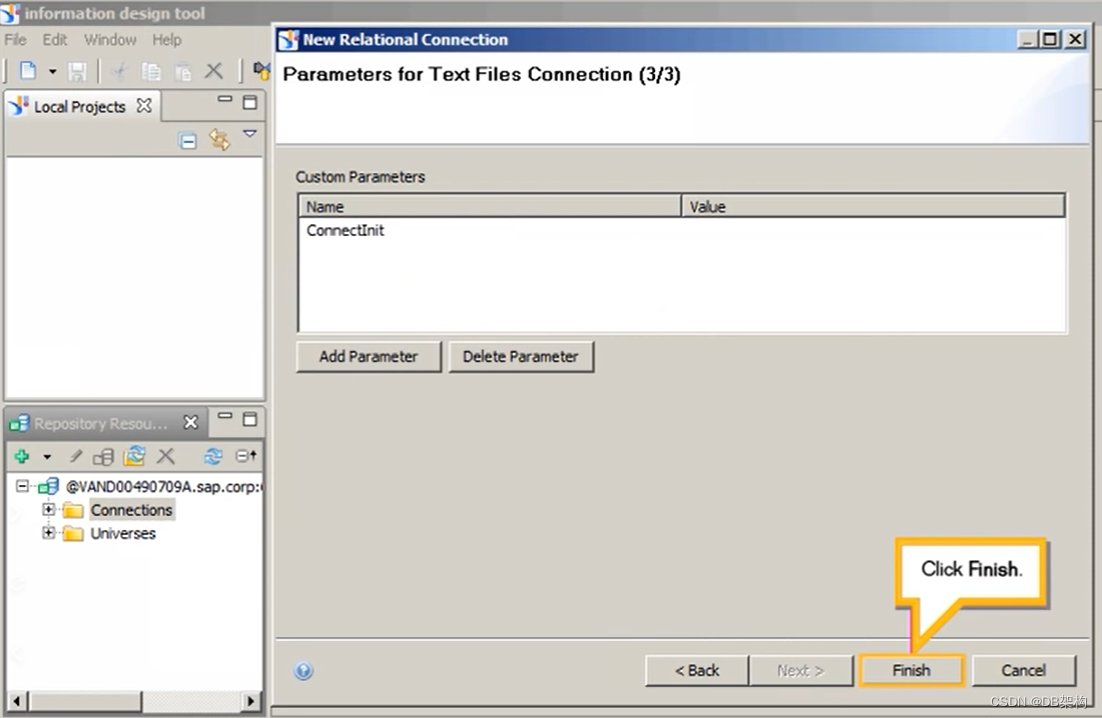
1.14 If desired, you can change the parameters for the connection. Click the Next>.
1.15 Click Finish.
1.16 Open the new connection and view the associated values. Click to expand the Connections folder.

1.17 Click to scroll down.

1.18 Double -click the Warehouse_csv connection.

1.19 Click the Show Values tab.

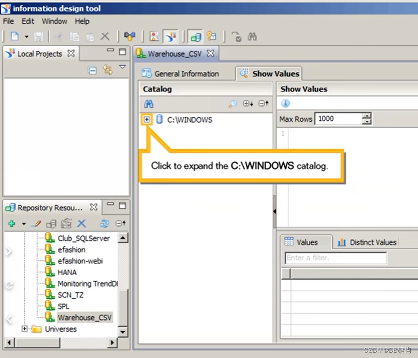
1.20 Click to expand the C:\WINDOWS catalog.
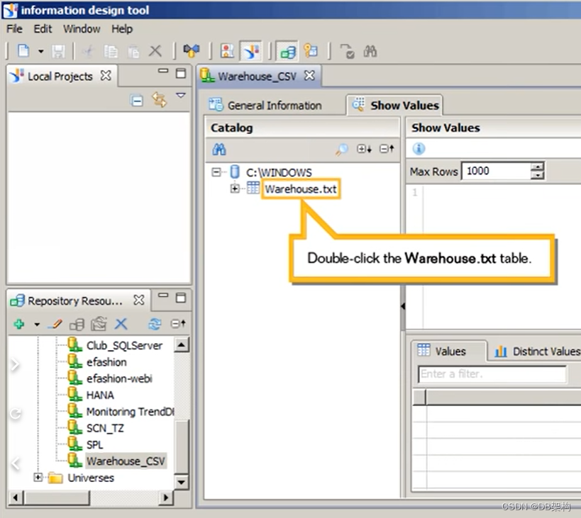
1.21 Double-click the Warehouse.txt table.
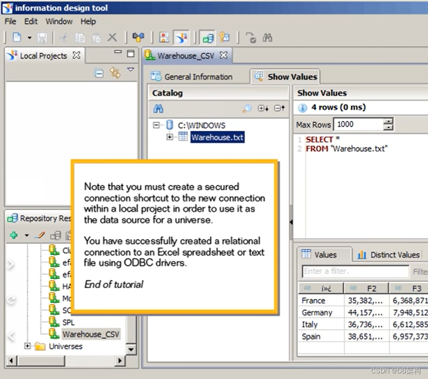
1.22 Note that you must create a secured connection shortcut to the new connection within a local project in order to use it as the data source for a universe.
2. Set aggregation navigation in a Business layer.
2.1 Click Actions From within the bussiness layer. Set aggregate navigation for the universe.

2.2 Select Set Aggregate Navigation...

2.3 Click Detect Incompatibility.

2.4 Clear the Imcompatible Objects Only check box.

2.5 Click Expand All

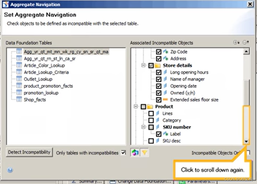
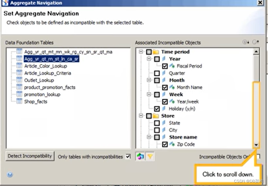
2.6 Click to scroll down.
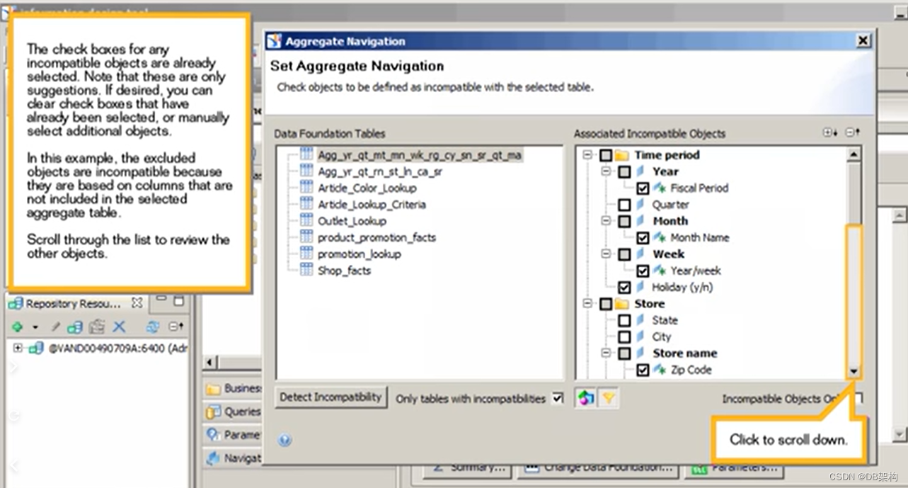
2.7 Click to scroll down again.
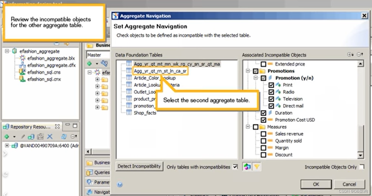
2.8 Select the second aggregate table.
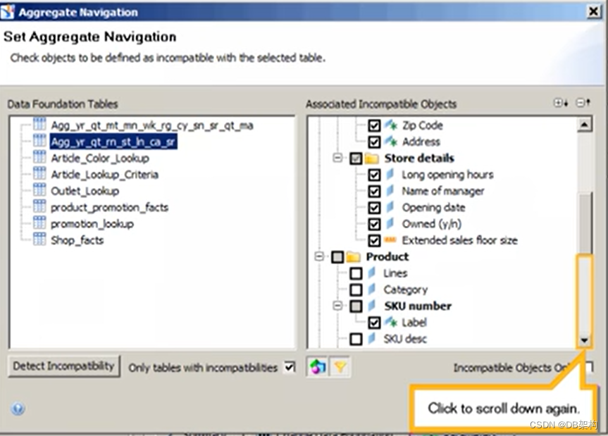
2.9 Click to scroll down.
2.10 Click to scroll down again.
2.11 Confirm the selected objects and save your changes, Click OK.
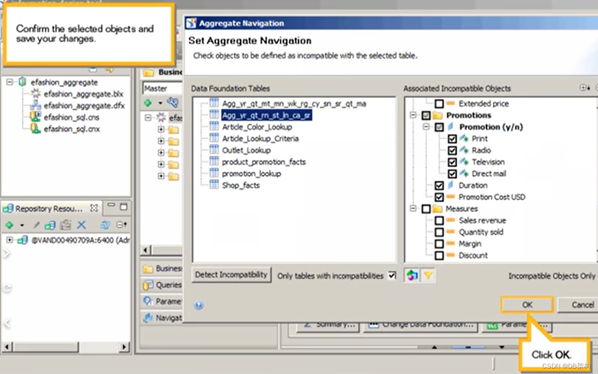
2.12 Click Save.

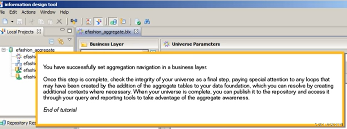
2.13 You have susccessfully set aggregation navigation in a bussiness layer.
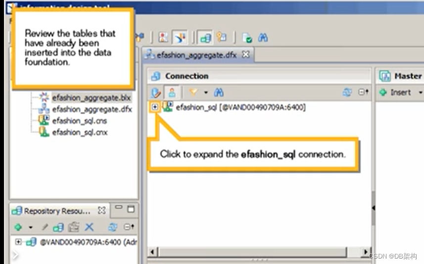
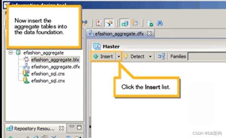
3. Insert aggregate table into a data foundation.
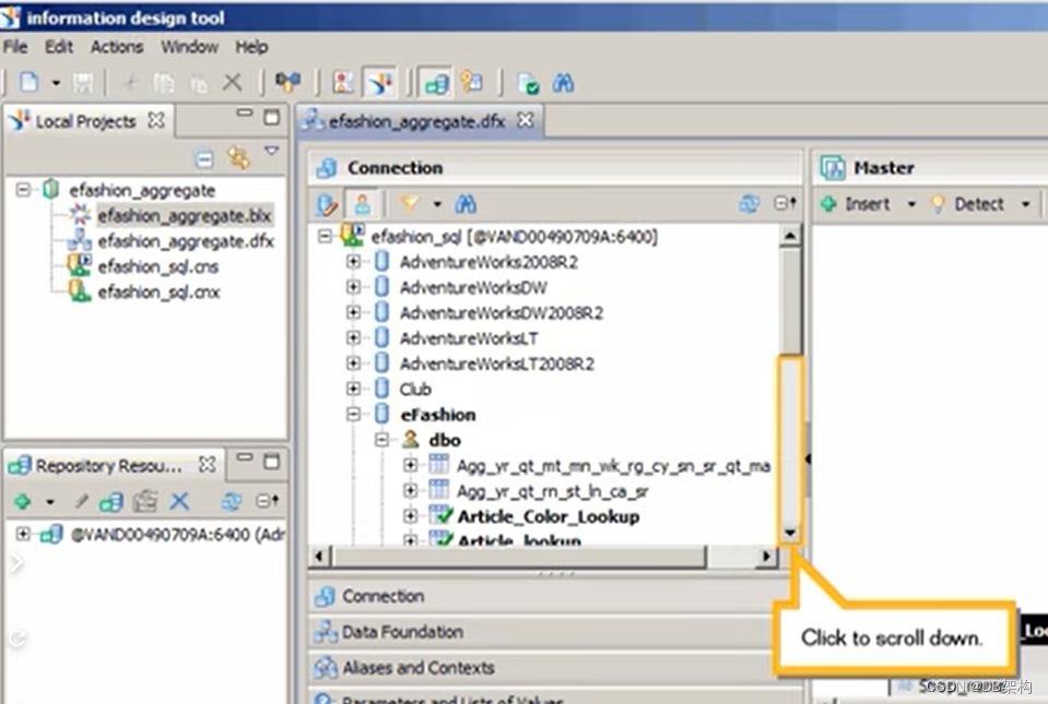
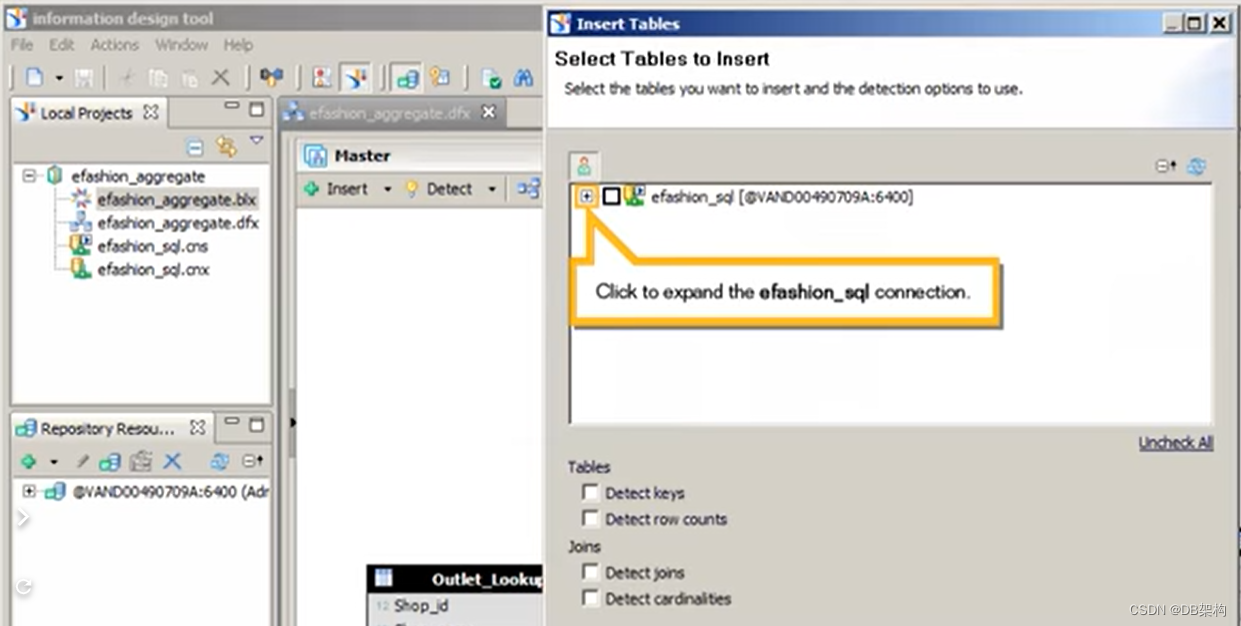
3.1 Click to expand the afashion_sql connection.
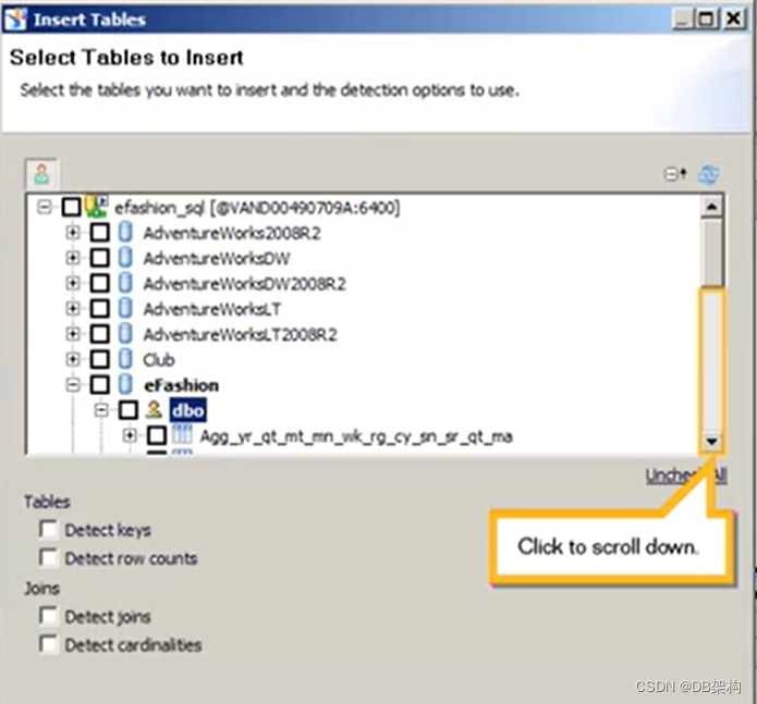
3.2Click to scroll down.
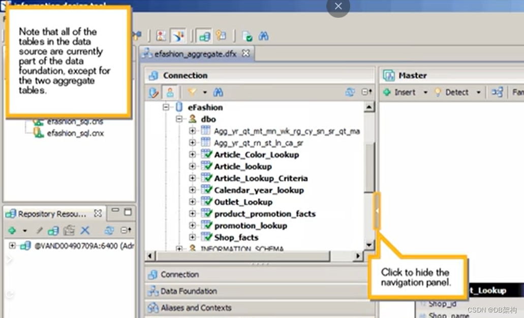
3.3 Click to hide the naviagtion panel.
3.4 Click the Insert list.
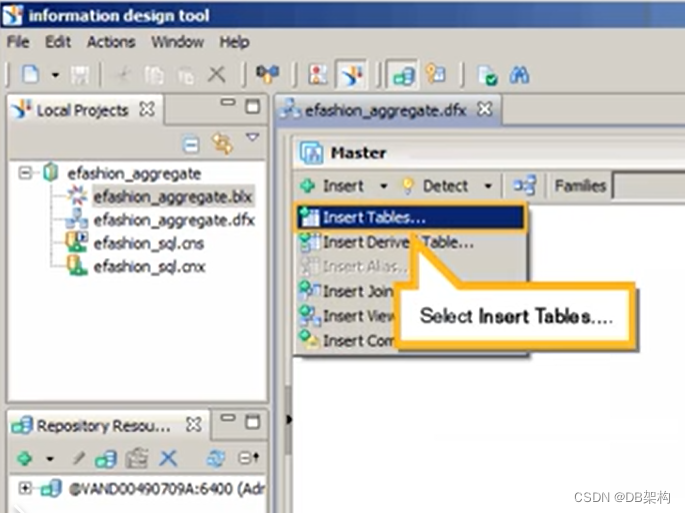
3.5 Select Insert Table...
3.6 Click to expand the afashion_sql connection.
3.7Click to scroll down.
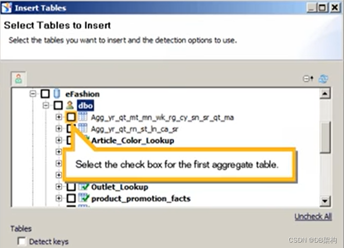
3.8 Select the check box for the first aggregate table.
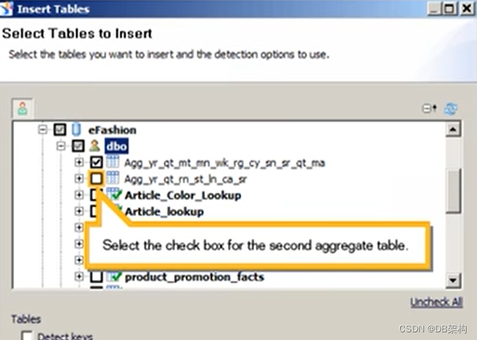
3.9 Select the check box for the second aggregate table.
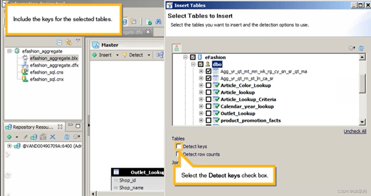
3.10 Select the Detect keys check box.
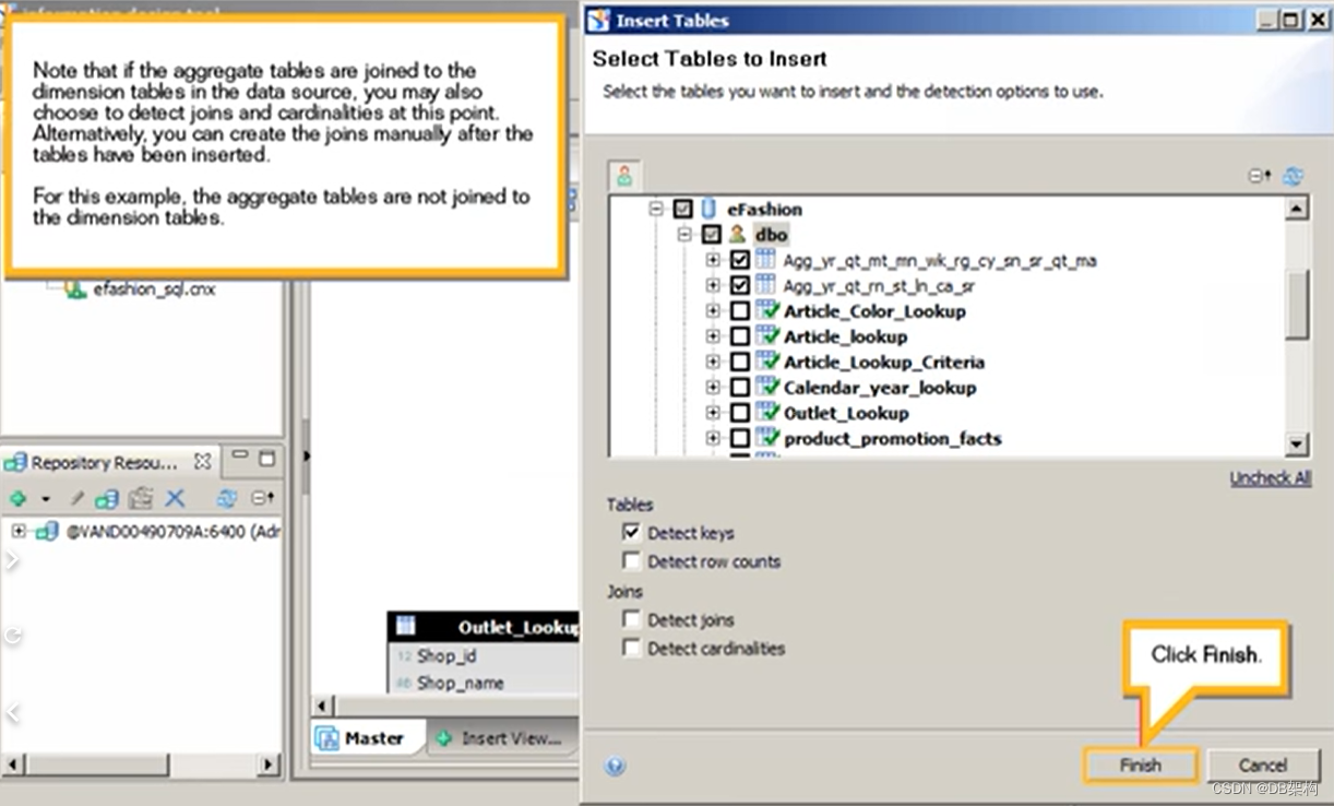
3.11 Click Finish.
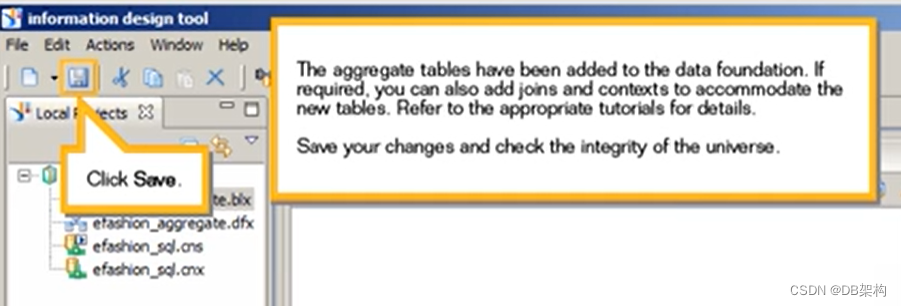
3.12 Click Save.
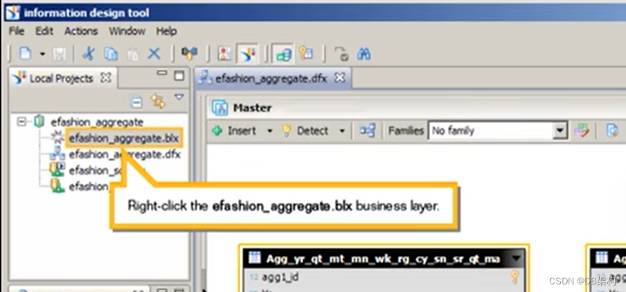
3.13 Right-click the efashion_aggregate .blx bussiness layer.
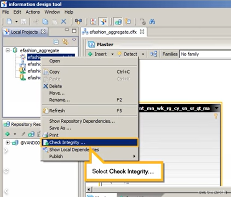
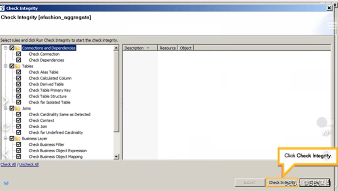
3.14 Select Check Integrity...
3.15 Click check all
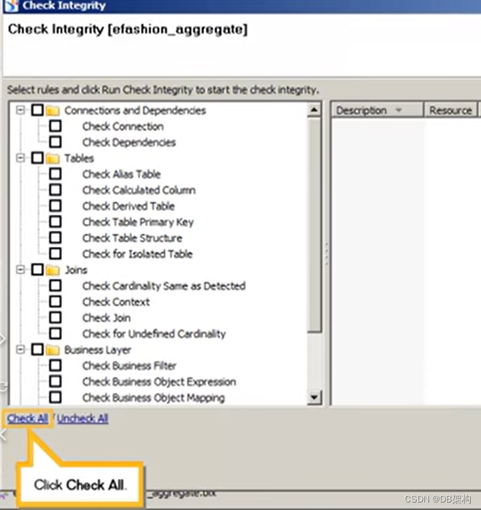
3.16 Click Check Intergrity.
3.17 Click Close.
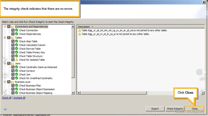
3.18 You have sucessfully inserted aggregate tables into a data foundation.
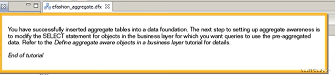
4. Define aggregate aware objects in a bussiness layer.
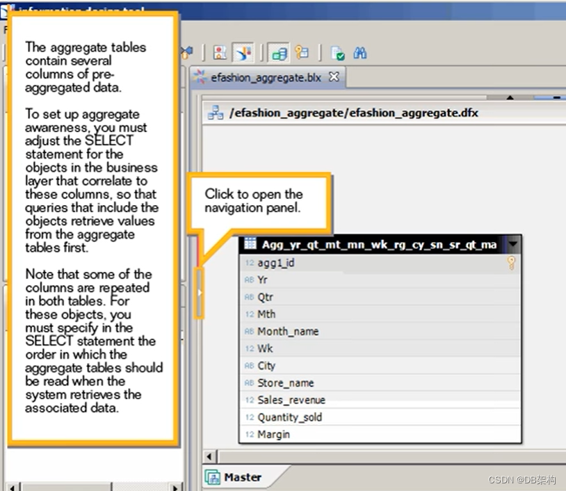
Once aggregate tables have been inserted into your data foundation. the next step to setting up aggregate awareness is a universe is to modify the SELECT statement of certain objects in the bussiness layer to make them aggregate aware.
In this tutorial, you will change the SELECT statements for both a dimension and a measure.
Note that this tutorial ware recored using SAP BusinessObjects information design tool 4.0 Feature Pack 3.
4.1 Click to open the navigation panel.
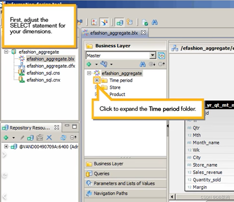
4.2 First , adjust the SELECT statement for your dimensions. Click to expand the Time period folder.
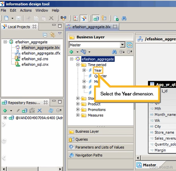
4.3 Select the Year dimension
4.4 Click SQL Assistant.

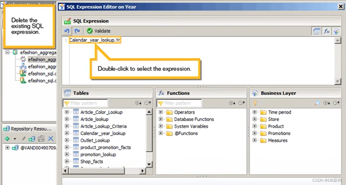
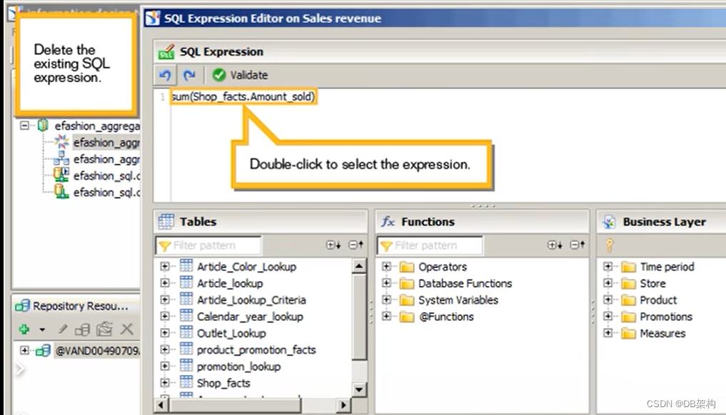
4.5 Double -click to select the expression.
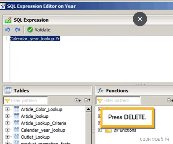
4.6 Press DELETE
4.7Click to expand the @Functions folder.
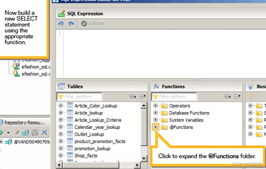
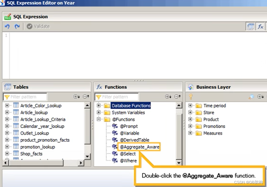
4.8 Double-Click the @Aggregate_Aware function.
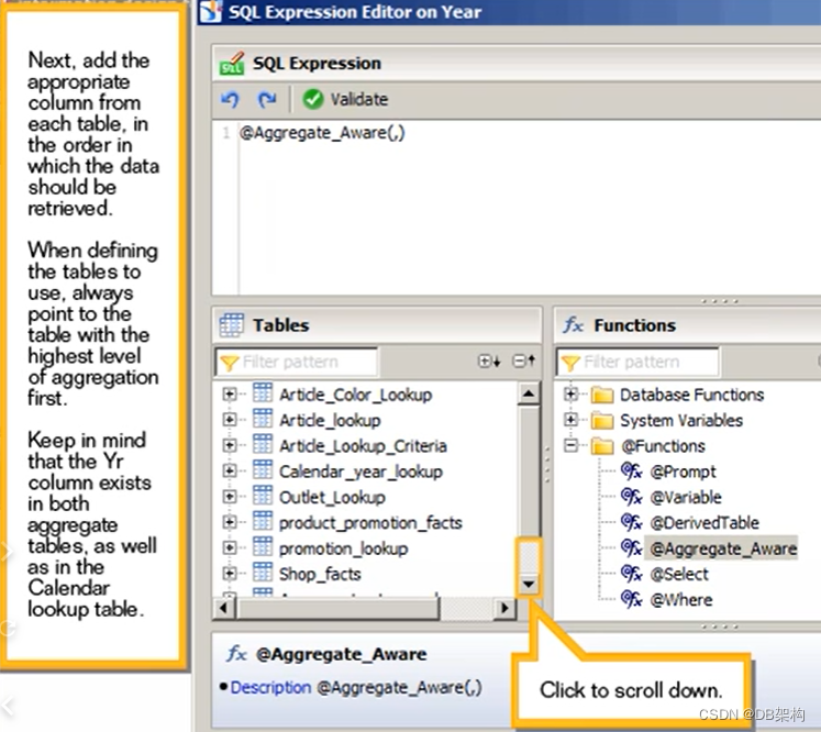
4.9 Click to scroll down.
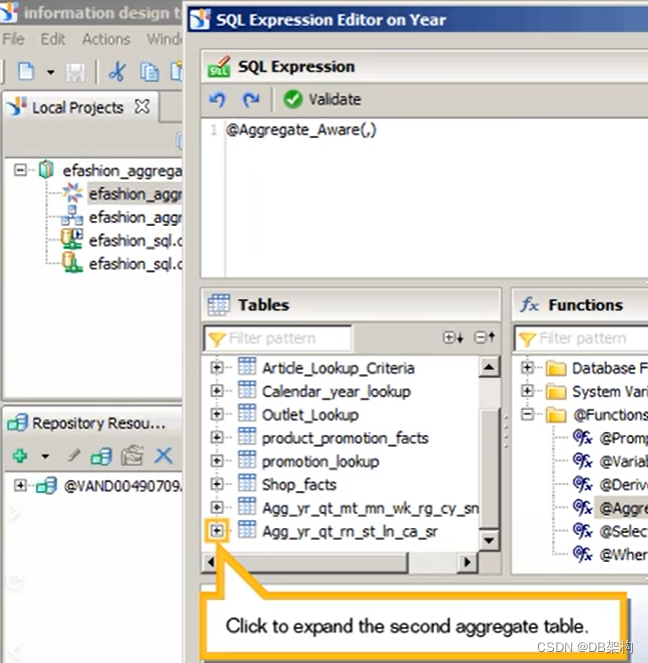
4.10 Click to expand the second aggregate table.
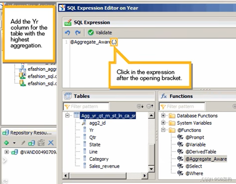
4.11 Add the Yr Column for the table with highest aggregation. Click in the expression after the opening bracket.
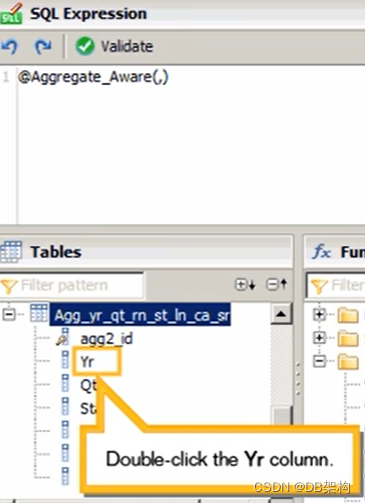
4.12 Double-click the Yr column.
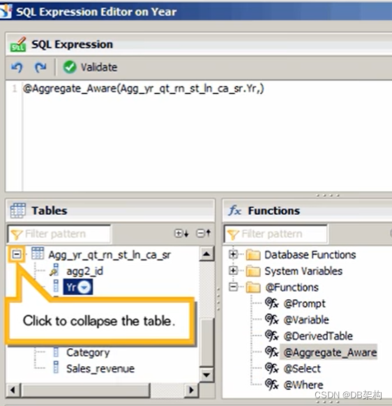
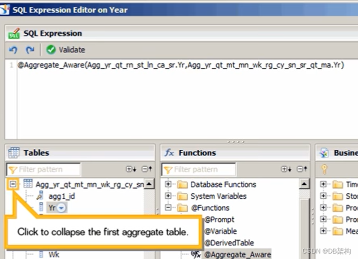
4.13 Click to collapse the table.
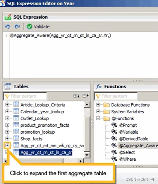
4.14 Click to expand the first aggregate table.
4.15 Add the same column for the next table.Click in the expression before the closing bracket.
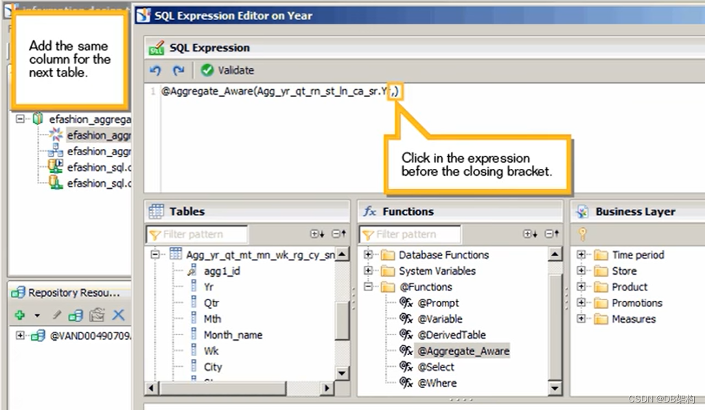
4.16 Double-click the Yr column.

4.17 Click to collapse the first aggregate table.
4.18 Click to expand the Calendar_year_lookup table.
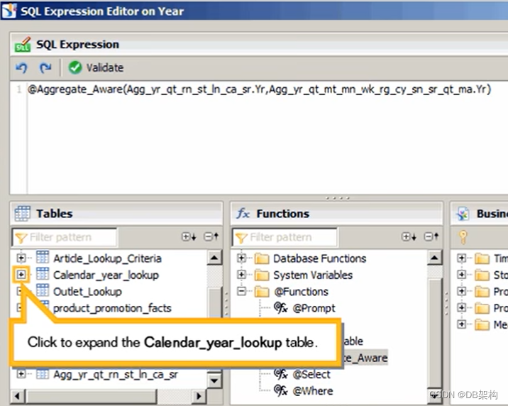
4.19 Click in the expression before the closing bracket.
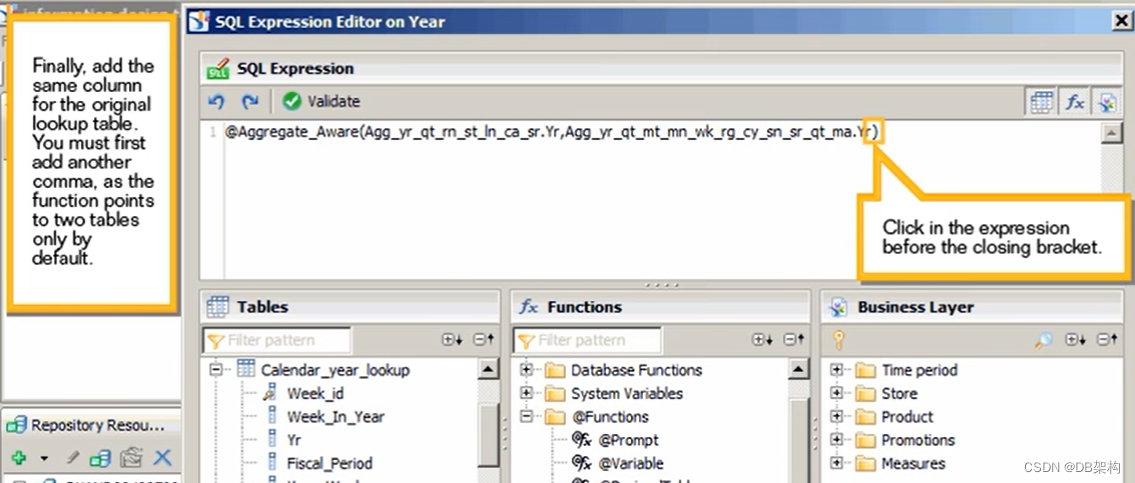
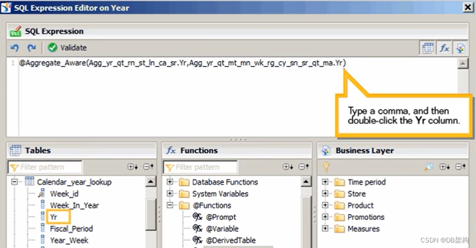
4.20 Type a comma,and then double-click the Yr column.
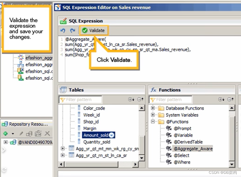
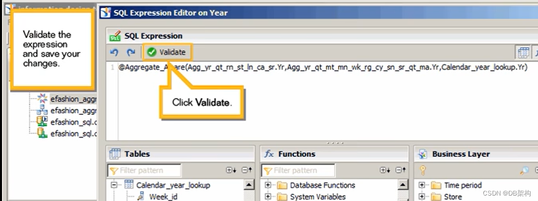
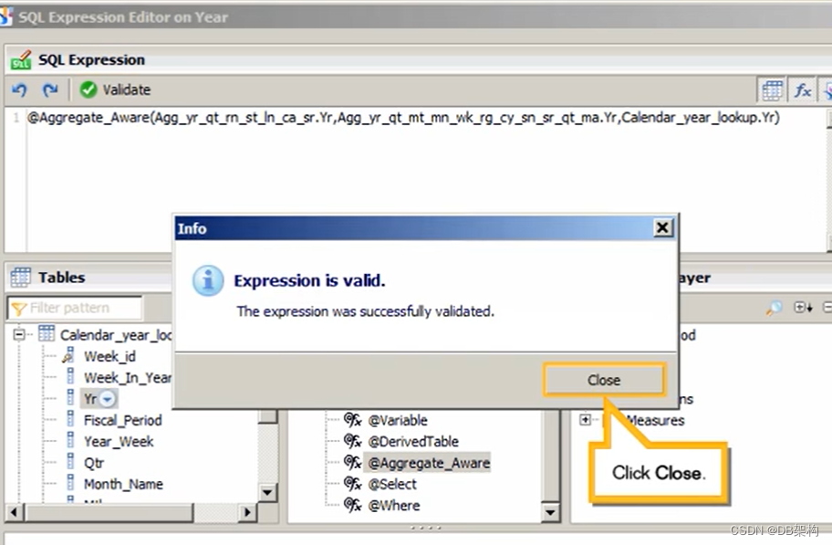
4.21 Validate the expression and save your changes. Click Validate.
4.22 Click Close
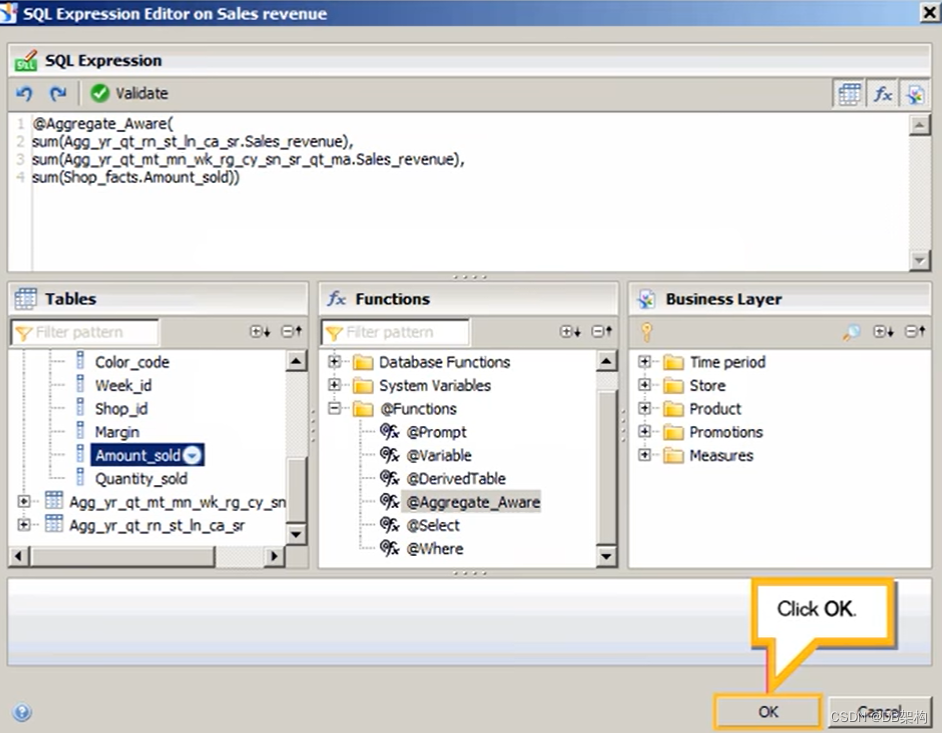
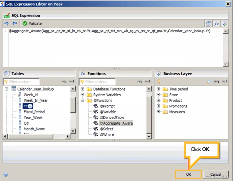
4.23 Click Ok
4.24 Click Save
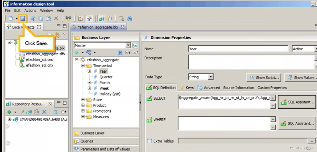
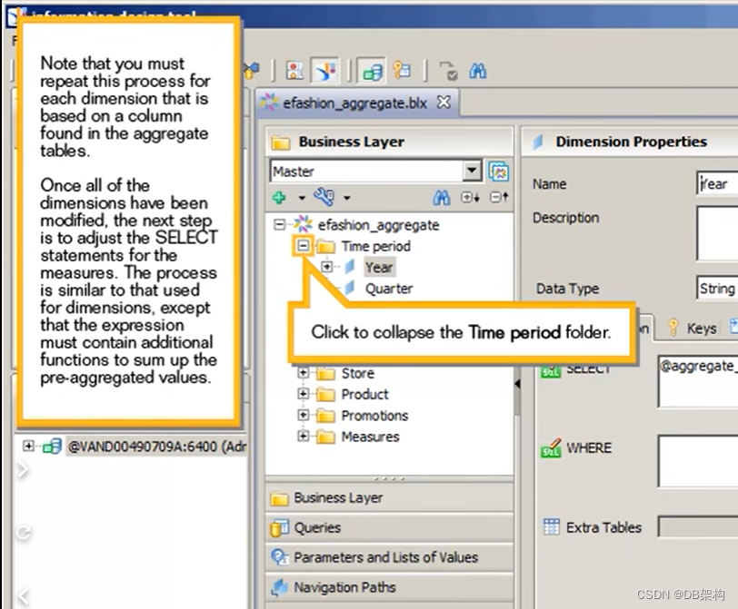
4.25 Click to collapse the Time period folder.
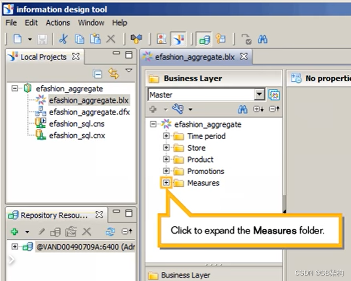
4.26 Click to expand the Measures folder.
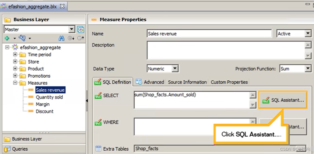
4.27 Select the Sales revenue measure.

4.28 Click SQL Assisant ...
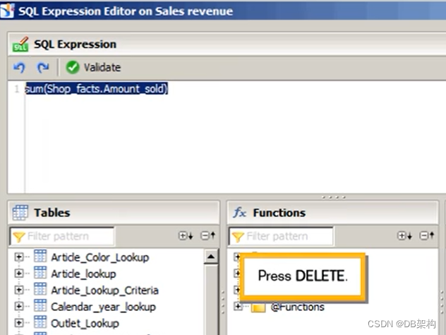
4.29 Double-click to select the expression. Press DELETE.
4.30 Add the appropriate function . Click to expand the @Function folder.

4.31 Double-click the @Aggregate_Aware function.

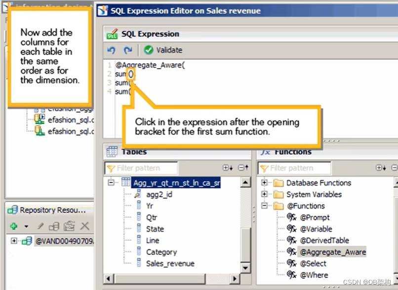
4.32 Click in the expression after the opening bracket.
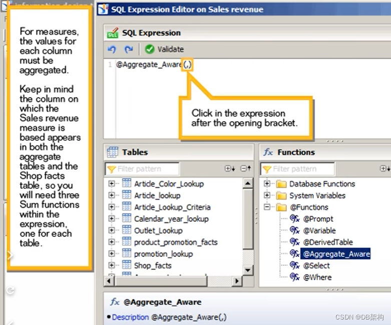
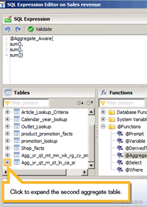
For mesures, the values for each column must be aggregated. Keep in mind the column on which the Sales revenue measure is based appears in both the aggregate tables and the Shop facts table, so you will need three Sum functions within the expression one for each table.
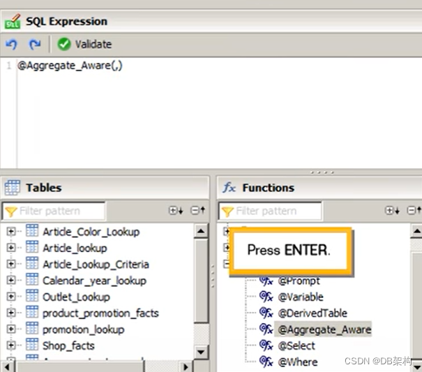
4.33 Press ENTER
4.34 Type sum(), and then press ENTER.

4.35 Type sum(),and then press ENTER again.

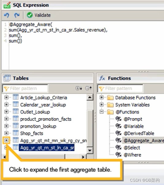
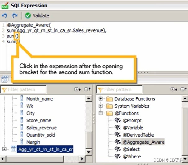
4.36 Type sum() and then click to scroll down.