- 随机数和蒙特卡洛模拟
- 求解单一变量非线性方程
- 求解线性系统方程
- 函数的数学积分
- 常微分方程的数值解
等势线绘图和曲线:
等势线 
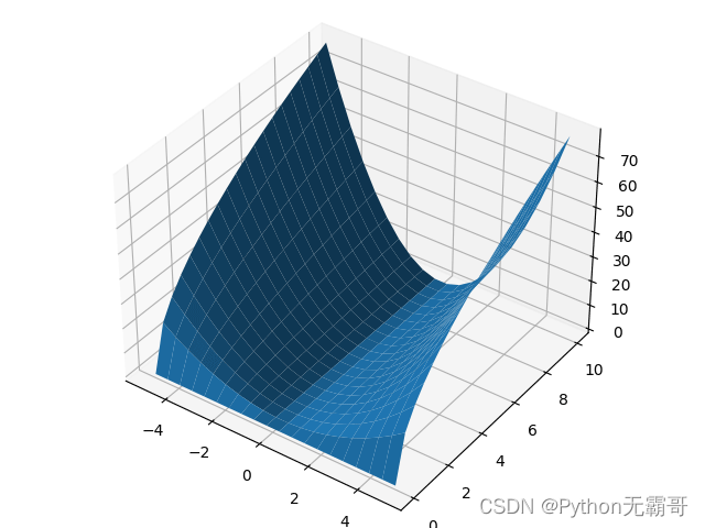
import numpy as np
import matplotlib.pyplot as plt
from mpl_toolkits.mplot3d import Axes3D

x_vals = np.linspace(-5,5,20)
y_vals = np.linspace(0,10,20)

X,Y = np.meshgrid(x_vals,y_vals)
Z = X**2 * Y**0.5
line_count = 15

ax = Axes3D(plt.figure())
ax.plot_surface(X,Y,Z,rstride=1,cstride=1)
plt.show()
非线性方程的数学解:
- 一般实函数 Scipy.optimize
- fsolve函数求零点(限定只给实数解)
import scipy.optimize as so
from scipy.optimize import fsolve

f = lambda x:x**2-1
fsolve(f,0.5)
fsolve(f,-0.5)
fsolve(f,[-0.5,0.5])


>>>fsolve(f,-0.5,full_output=True)
>>>(array([-1.]), {

    'nfev': 9, 'fjac': array([[-1.]]), 'r': array([1.99999875]), 'qtf': array([3.82396337e-10]), 'fvec': array([4.4408921e-16])}, 1, 'The solution converged.')

>>>help(fsolve)
>>>Help on function fsolve in module scipy.optimize._minpack_py:

fsolve(func, x0, args=(), fprime=None, full_output=0, col_deriv=0, xtol=1.49012e-08, maxfev=0, band=None, epsfcn=None, factor=100, diag=None)
    Find the roots of a function.

    Return the roots of the (non-linear) equations defined by
    ``func(x) = 0`` given a starting estimate.

    Parameters
    ----------
    func : callable ``f(x, *args)``
        A function that takes at least one (possibly vector) argument,
        and returns a value of the same length.
    x0 : ndarray
        The starting estimate for the roots of ``func(x) = 0``.
    args : tuple, optional
        Any extra arguments to `func`.
    fprime : callable ``f(x, *args)``, optional
        A function to compute the Jacobian of `func` with derivatives
        across the rows. By default, the Jacobian will be estimated.
    full_output : bool, optional
        If True, return optional outputs.
    col_deriv : bool, optional
        Specify whether the Jacobian function computes derivatives down
        the columns (faster, because there is no transpose operation).
    xtol : float, optional
        The calculation will terminate if the relative error between two
        consecutive iterates is at most `xtol`.
    maxfev : int, optional
        The maximum number of calls to the function. If zero, then
        ``100*(N+1)`` is the maximum where N is the number of elements
        in `x0`.
    band : tuple, optional
        If set to a two-sequence containing the number of sub- and
        super-diagonals within the band of the Jacobi matrix, the
        Jacobi matrix is considered banded (only for ``fprime=None``).
    epsfcn : float, optional
        A suitable step length for the forward-difference
        approximation of the Jacobian (for ``fprime=None``). If
        `epsfcn` is less than the machine precision, it is assumed
        that the relative errors in the functions are of the order of
        the machine precision.
    factor : float, optional
        A parameter determining the initial step bound
        (``factor * || diag * x||``). Should be in the interval
        ``(0.1, 100)``.
    diag : sequence, optional
        N positive entries that serve as a scale factors for the
        variables.

    Returns
    -------
    x : ndarray
        The solution (or the result of the last iteration for
        an unsuccessful call).
    infodict : dict
        A dictionary of optional outputs with the keys:

        ``nfev``
            number of function calls
        ``njev``
            number of Jacobian calls
        ``fvec``
            function evaluated at the output
        ``fjac``
            the orthogonal matrix, q, produced by the QR
            factorization of the final approximate Jacobian
            matrix, stored column wise
        ``r``
            upper triangular matrix produced by QR factorization
            of the same matrix
        ``qtf``
            the vector ``(transpose(q) * fvec)``

    ier : int
        An integer flag.  Set to 1 if a solution was found, otherwise refer
        to `mesg` for more information.
    mesg : str
        If no solution is found, `mesg` details the cause of failure.

    See Also
    --------
    root : Interface to root finding algorithms for multivariate
           functions. See the ``method=='hybr'`` in particular.

    Notes
    -----
    ``fsolve`` is a wrapper around MINPACK's hybrd and hybrj algorithms.

    Examples
    --------
    Find a solution to the system of equations:
    ``x0*cos(x1) = 4,  x1*x0 - x1 = 5``.

    >>> from scipy.optimize import fsolve
    >>> def func(x):
    ...     return [x[0] * np.cos(x[1]) - 4,
    ...             x[1] * x[0] - x[1] - 5]
    >>> root = fsolve(func, [1, 1])
    >>> root
    array([6.50409711, 0.90841421])
    >>> np.isclose(func(root), [0.0, 0.0])  # func(root) should be almost 0.0.
    array([ True,  True])
关键字参数: full_output=True
多项式的复数根 :np.roots([最高位系数,次高位系数,… … x项系数,常数项])
>>>f = lambda x:x**4 + x -1
>>>np.roots([1,0,0,1,-1])
>>>array([-1.22074408+0.j        ,  0.24812606+1.03398206j,
        0.24812606-1.03398206j,  0.72449196+0.j        ])
- 求解线性等式 scipy.linalg
- 利用dir()获取常用函数
import numpy as np
import scipy.linalg as sla
from scipy.linalg import inv
a = np.array([-1,5])
c = np.array([[1,3],[3,4]])
x = np.dot(inv(c),a)

>>>x
>>>array([ 3.8, -1.6])
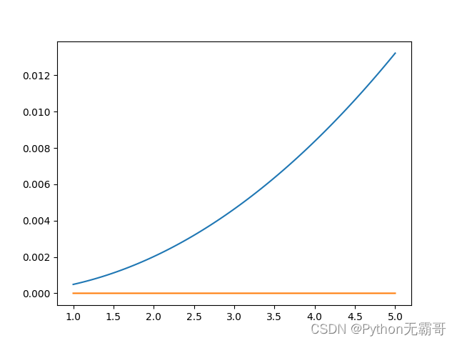
数值积分 scipy.integrate
- 利用dir()获取你需要的信息
- 对自定义函数做积分
import scipy.integrate as si
from scipy.integrate import quad
import numpy as np
import matplotlib.pyplot as plt
f = lambda x:x**1.05*0.001

interval = 100
xmax = np.linspace(1,5,interval)
integral,error = np.zeros(xmax.size),np.zeros(xmax.size)
for i in range(interval):
    integral[i],error[i] = quad(f,0,xmax[i])
plt.plot(xmax,integral,label="integral")
plt.plot(xmax,error,label="error")
plt.show()
对震荡函数做积分
quad 函数允许 调整他使用的网格
>>>(-0.4677718053224297, 2.5318630220102742e-05)
>>>quad(np.cos,-1,1,limit=100)
>>>(1.6829419696157932, 1.8684409237754643e-14)
>>>quad(np.cos,-1,1,limit=1000)
>>>(1.6829419696157932, 1.8684409237754643e-14)
>>>quad(np.cos,-1,1,limit=10)
>>>(1.6829419696157932, 1.8684409237754643e-14)
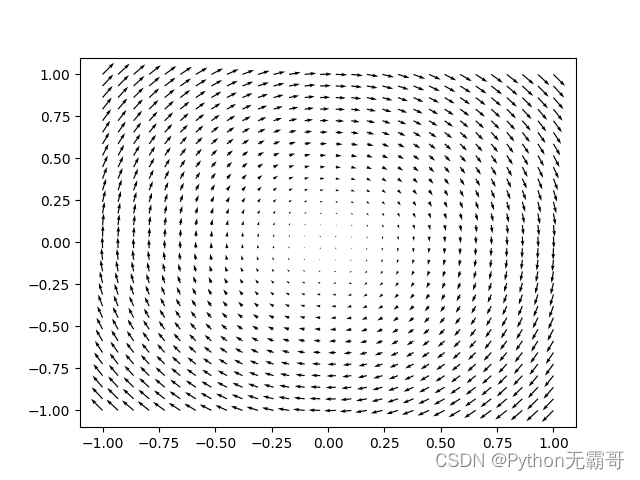
向量场与流线图:
vector(x,y) = (y,-x)
import numpy as np
import matplotlib.pyplot as plt
coords = np.linspace(-1,1,30)
X,Y = np.meshgrid(coords,coords)
Vx,Vy = Y,-X
plt.quiver(X,Y,Vx,Vy)
plt.show()
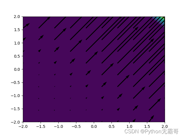
------------------
import numpy as np
import matplotlib.pyplot as plt
coords = np.linspace(-2,2,10)
X,Y = np.meshgrid(coords,coords)
Z = np.exp(np.exp(X+Y))
ds = 4/6
dX,dY = np.gradient(Z,ds)
plt.contourf(X,Y,Z,25)
plt.quiver(X,Y,dX.transpose(),dY.transpose(),scale=25)
plt.show()