OpenFOAM的vtk流场文件的Python后处理脚本-以统计轴向固含率为例

实现了用python处理OpenFOAM生成的vtk流场文件的脚本。
1、流场生成vtk文件， reconstructPar， foamToVTK -ascii, 结果放在./VTK文件夹下

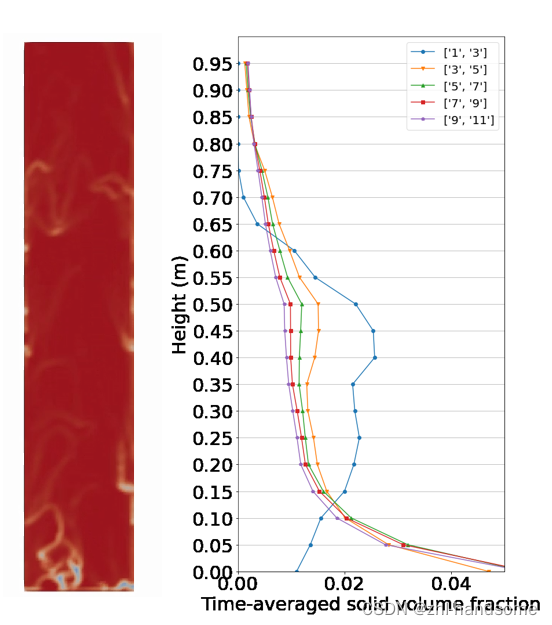
2、运行后处理脚本，目前只支持网格大小相等的结构网格，可以全自动生成轴向固含率分布图和数据。

3、需要时变数据只需将下面脚本改为函数即可。

import vtk
import numpy as np
import matplotlib.pyplot as plt
import matplotlib as mpl

reader = vtk.vtkUnstructuredGridReader()
reader.SetFileName("./VTK/cfd_100.vtk")
reader.Update()
output = reader.GetOutput()
# print(output)

points = output.GetPoints()
voidfractions = output.GetCellData().GetArray("voidfractionMean")

cell_centers = vtk.vtkCellCenters()
cell_centers.SetInputData(output)
cell_centers.Update()


# point = points.GetPoint(1)
# point = output.GetPoint(1)
# point, voidfraction
# # ((0.004999999888241291, 0.0, 0.0), 0.9999974966049194)

points_np = np.array([points.GetPoint(i) for i in range(points.GetNumberOfPoints())])
voidfractions_np = np.array([voidfractions.GetValue(i) for i in range(voidfractions.GetNumberOfTuples())])

cell_centers_np = np.array([cell_centers.GetOutput().GetPoint(i) for i in range(cell_centers.GetOutput().GetNumberOfPoints())])

zLength = max(points_np[:,2])
gap = zLength/20
threshold = gap/2
# volume = 6.25e-9
volume = 1
heights = np.arange(0, 1, gap)
solid_volume_fractions = []
height_of_data = []
z_index = 2
cell_number = cell_centers.GetOutput().GetNumberOfPoints()

for height in heights:
    # print(height)
    num_of_points = 0
    total_volume = 0
    solid_volume = 0
    
    for i in range(0, cell_number):
        if cell_centers_np[i][z_index] >= height - threshold and cell_centers_np[i][z_index] <= height + threshold:
            num_of_points += 1
            total_volume += volume
            solid_volume += volume * (1 - voidfractions_np[i])
            
    if not num_of_points == 0:
        height_of_data.append(height)
        solid_volume_fractions.append(solid_volume / total_volume)

print('drawing solid volume fraction')
sizefactor = 1.2
fig = plt.figure(figsize=(10 / sizefactor, 20/ sizefactor))
# plt.subplots_adjust(top=0.96, bottom=0.08, left=0.14, right=0.92)
plt.subplots_adjust(top=0.96, bottom=0.1)
ax = fig.subplots()
ax.plot(solid_volume_fractions, height_of_data, marker='o')
ax.grid(axis='y')
ax.set_ylabel('Height (m)', fontsize=22)
ax.set_xlabel('Time-averaged solid volume fraction', fontsize=22)
plt.tick_params(labelsize=16)
# xtick = np.arange(0, 0.5, 0.05)
# ax.set_xticks(xtick)
# ytick = np.arange(0, 60, 5)
# ax.set_yticks(ytick)
# ax.set_xlim(0, 0.5)
# ax.set_ylim(0, 1)
# plt.savefig('solid_volume_fraction.png')
plt.show()
plt.close()

# output data
with open('solid_volume_fraction.dat', 'w') as f_obj:
    for i in range(0, len(height_of_data)):
        f_obj.write('%f   %f\n' % (height_of_data[i], solid_volume_fractions[i]))

结果展示：