文章目录
数据可视化第二版-03部分-09章-时间趋势
总结
本系列博客为基于《数据可视化第二版》一书的教学资源博客。本文主要是第9章,时间趋势可视化的案例相关。
可视化视角-时间趋势


代码实现
安装依赖
pip install scikit-learn -i https://pypi.tuna.tsinghua.edu.cn/simple
pip install seaborn -i https://pypi.tuna.tsinghua.edu.cn/simple
pip install tushare==1.2.89 -i https://pypi.tuna.tsinghua.edu.cn/simple
pip install mplfinance==0.12.9b7 -i https://pypi.tuna.tsinghua.edu.cn/simple
折线图
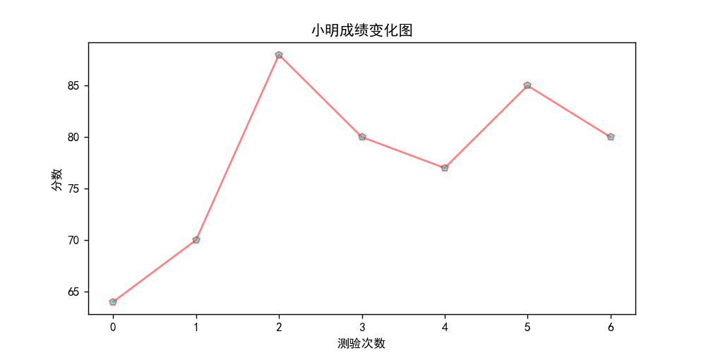
折线图1
# 折线图实现1
import matplotlib.pyplot as plt

# 解决中文乱码问题
plt.rcParams['font.sans-serif'] = ['SimHei']
# X轴,Y轴数据
x = [0, 1, 2, 3, 4, 5, 6]
y = [64, 70, 88, 80, 77, 85, 80]
plt.figure(figsize=(8, 4))  # 创建绘图对象
# 在当前绘图对象绘图,设置曲线参数(X轴,Y轴,红色实线,线宽度)
plt.plot(x, y, color="r", marker="p", linestyle="-", alpha=0.5, mfc="c")
plt.xlabel("测验次数")  # X轴标签
plt.ylabel("分数")  # Y轴标签
plt.title("小明成绩变化图")  # 图标题
plt.show()  # 显示图
输出为:
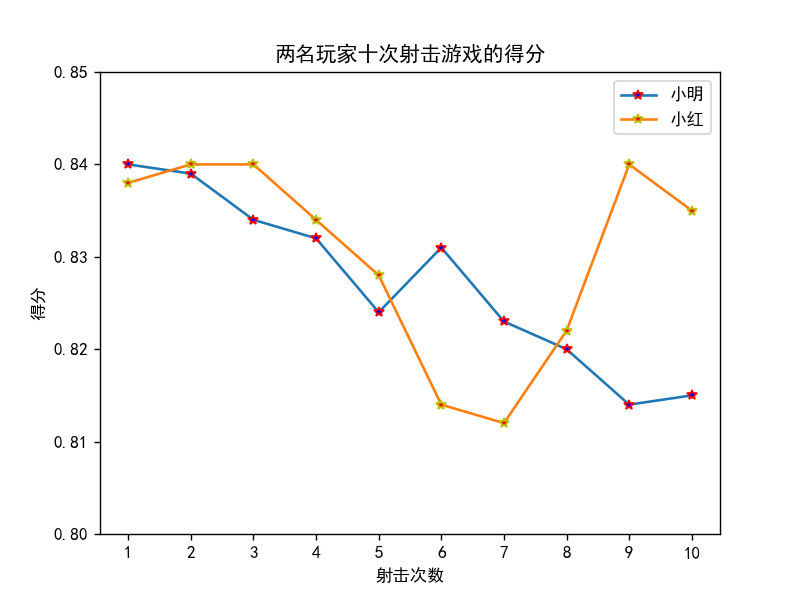
折线图案例2
# 折线图实现二
import matplotlib.pyplot as plt

plt.rcParams['font.sans-serif'] = ['SimHei']  # 解决中文乱码问题
x = range(1, 11)
y1 = [0.840, 0.839, 0.834, 0.832, 0.824, 0.831, 0.823, 0.820, 0.814, 0.815]
y2 = [0.838, 0.840, 0.840, 0.834, 0.828, 0.814, 0.812, 0.822, 0.840, 0.835]
plt.plot(x, y1, marker='*', mec='r', mfc='b', label='小明')
plt.plot(x, y2, marker='*', mec='y', mfc='r', label='小红')
plt.legend()  # 让图例生效
plt.xticks(x, rotation=1)
plt.xlabel('射击次数')  # X轴标签
plt.ylabel("得分")  # Y轴标签
plt.ylim(0.8, 0.85)
plt.title("两名玩家十次射击游戏的得分")  # 标题
plt.show()
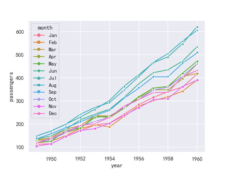
折线图示例3-seaborn
参考:https://blog.csdn.net/m0_38139250/article/details/129729191
import numpy as np
import pandas as pd
import matplotlib.pyplot as plt
import matplotlib as  mpl
import seaborn as sns
sns.set_theme(style="darkgrid")

mpl.rcParams['font.sans-serif']=['SimHei']
mpl.rcParams['axes.unicode_minus']=False

flights = sns.load_dataset("flights",cache=True,data_home=r'.\seaborn-data')
flights.head()
#使用标记而不是破折号来识别组
ax = sns.lineplot(x="year", y="passengers",hue="month", style="month",
markers=True, dashes=False, data=flights)

plt.show()
面积图
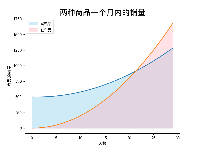
面积图1-堆叠面积图
# 堆叠面积图

from matplotlib import pyplot as plt

plt.rcParams['font.sans-serif'] = ['SimHei']  # 解决中文乱码问题
x = [i for i in range(30)]
y1 = [x ** 2 - 2 * x + 500 for x in range(30)]
y2 = [2 * x ** 2 for x in range(30)]
plt.plot(x, y1)
plt.plot(x, y2)
plt.fill_between(x, y1, color='skyblue', alpha=0.4, label='A产品')
plt.fill_between(x, y2, color='lightpink', alpha=0.4, label='B产品')
plt.xlabel('天数')
plt.ylabel('商品的销量')
plt.title('两种商品一个月内的销量', fontsize=18)
plt.legend()  # 让图例生效
plt.show()
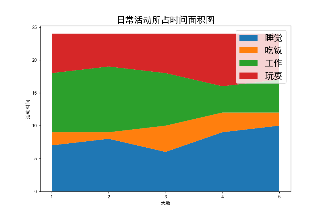
面积图2-堆积面积图
# 堆叠面积图
import matplotlib.pyplot as plt

plt.rcParams['font.sans-serif'] = ['SimHei']  # 解决中文乱码问题
days = [1, 2, 3, 4, 5]
sleeping = [7, 8, 6, 9, 10]
eating = [2, 1, 4, 3, 2]
working = [9, 10, 8, 4, 5]
playing = [6, 5, 6, 8, 7]
plt.figure(figsize=(9, 6))
plt.stackplot(days, sleeping, eating, working, playing)
plt.xlabel('天数')
plt.ylabel('活动时间')
plt.xticks([1, 2, 3, 4, 5])
plt.title('日常活动所占时间面积图', fontsize=18)
plt.legend(['睡觉', '吃饭', '工作', '玩耍'], fontsize=18)
plt.show()
河流图
参考:
Themeriver - Theme_river
ThemeRiver:主题河流图
河流图1
# 社团招新河流图
import pyecharts.options as opts
from pyecharts.charts import ThemeRiver

x_data = ["书画协会", "嘻哈社", "厨艺社"]
y_data = [
    ["2018/09/01", 10, "书画协会"],
    ["2019/09/01", 1, "书画协会"],
    ["2020/09/01", 3, "书画协会"],
    ["2018/09/01", 1, "嘻哈社"],
    ["2019/09/01", 2, "嘻哈社"],
    ["2020/09/01", 3, "嘻哈社"],
    ["2018/09/01", 4, "厨艺社"],
    ["2019/09/01", 5, "厨艺社"],
    ["2020/09/01", 6, "厨艺社"],
]
(
    ThemeRiver(init_opts=opts.InitOpts(width="1000px", height="500px"))
        .add(
        series_name=x_data,
        data=y_data,
        singleaxis_opts=opts.SingleAxisOpts(
            pos_top="50", pos_bottom="50", type_="time"
        ),
    )
        .set_global_opts(
        tooltip_opts=opts.TooltipOpts(trigger="axis", axis_pointer_type="line")
    )
        .render("社团招新人数河流图.html")
)

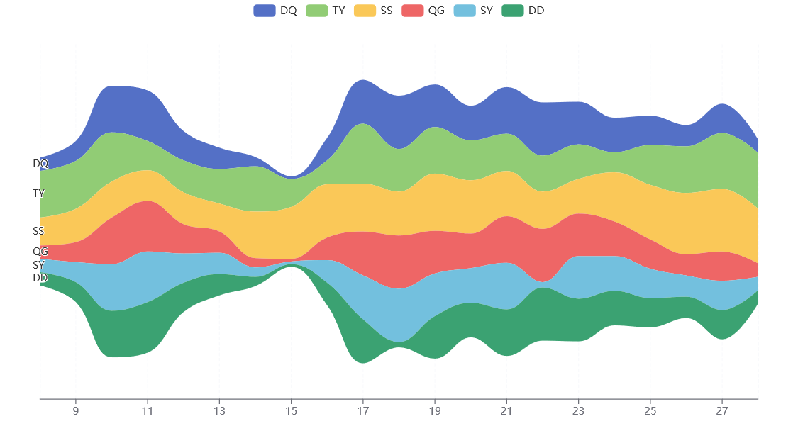
河流图2
import pyecharts.options as opts
from pyecharts.charts import ThemeRiver

"""
Gallery 使用 pyecharts 1.1.0
参考地址: https://echarts.apache.org/examples/editor.html?c=themeRiver-basic

目前无法实现的功能:

1、暂时无法设置阴影样式
"""
x_data = ["DQ", "TY", "SS", "QG", "SY", "DD"]
y_data = [
    ["2015/11/08", 10, "DQ"],
    ["2015/11/09", 15, "DQ"],
    ["2015/11/10", 35, "DQ"],
    ["2015/11/11", 38, "DQ"],
    ["2015/11/12", 22, "DQ"],
    ["2015/11/13", 16, "DQ"],
    ["2015/11/14", 7, "DQ"],
    ["2015/11/15", 2, "DQ"],
    ["2015/11/16", 17, "DQ"],
    ["2015/11/17", 33, "DQ"],
    ["2015/11/18", 40, "DQ"],
    ["2015/11/19", 32, "DQ"],
    ["2015/11/20", 26, "DQ"],
    ["2015/11/21", 35, "DQ"],
    ["2015/11/22", 40, "DQ"],
    ["2015/11/23", 32, "DQ"],
    ["2015/11/24", 26, "DQ"],
    ["2015/11/25", 22, "DQ"],
    ["2015/11/26", 16, "DQ"],
    ["2015/11/27", 22, "DQ"],
    ["2015/11/28", 10, "DQ"],
    ["2015/11/08", 35, "TY"],
    ["2015/11/09", 36, "TY"],
    ["2015/11/10", 37, "TY"],
    ["2015/11/11", 22, "TY"],
    ["2015/11/12", 24, "TY"],
    ["2015/11/13", 26, "TY"],
    ["2015/11/14", 34, "TY"],
    ["2015/11/15", 21, "TY"],
    ["2015/11/16", 18, "TY"],
    ["2015/11/17", 45, "TY"],
    ["2015/11/18", 32, "TY"],
    ["2015/11/19", 35, "TY"],
    ["2015/11/20", 30, "TY"],
    ["2015/11/21", 28, "TY"],
    ["2015/11/22", 27, "TY"],
    ["2015/11/23", 26, "TY"],
    ["2015/11/24", 15, "TY"],
    ["2015/11/25", 30, "TY"],
    ["2015/11/26", 35, "TY"],
    ["2015/11/27", 42, "TY"],
    ["2015/11/28", 42, "TY"],
    ["2015/11/08", 21, "SS"],
    ["2015/11/09", 25, "SS"],
    ["2015/11/10", 27, "SS"],
    ["2015/11/11", 23, "SS"],
    ["2015/11/12", 24, "SS"],
    ["2015/11/13", 21, "SS"],
    ["2015/11/14", 35, "SS"],
    ["2015/11/15", 39, "SS"],
    ["2015/11/16", 40, "SS"],
    ["2015/11/17", 36, "SS"],
    ["2015/11/18", 33, "SS"],
    ["2015/11/19", 43, "SS"],
    ["2015/11/20", 40, "SS"],
    ["2015/11/21", 34, "SS"],
    ["2015/11/22", 28, "SS"],
    ["2015/11/23", 26, "SS"],
    ["2015/11/24", 37, "SS"],
    ["2015/11/25", 41, "SS"],
    ["2015/11/26", 46, "SS"],
    ["2015/11/27", 47, "SS"],
    ["2015/11/28", 41, "SS"],
    ["2015/11/08", 10, "QG"],
    ["2015/11/09", 15, "QG"],
    ["2015/11/10", 35, "QG"],
    ["2015/11/11", 38, "QG"],
    ["2015/11/12", 22, "QG"],
    ["2015/11/13", 16, "QG"],
    ["2015/11/14", 7, "QG"],
    ["2015/11/15", 2, "QG"],
    ["2015/11/16", 17, "QG"],
    ["2015/11/17", 33, "QG"],
    ["2015/11/18", 40, "QG"],
    ["2015/11/19", 32, "QG"],
    ["2015/11/20", 26, "QG"],
    ["2015/11/21", 35, "QG"],
    ["2015/11/22", 40, "QG"],
    ["2015/11/23", 32, "QG"],
    ["2015/11/24", 26, "QG"],
    ["2015/11/25", 22, "QG"],
    ["2015/11/26", 16, "QG"],
    ["2015/11/27", 22, "QG"],
    ["2015/11/28", 10, "QG"],
    ["2015/11/08", 10, "SY"],
    ["2015/11/09", 15, "SY"],
    ["2015/11/10", 35, "SY"],
    ["2015/11/11", 38, "SY"],
    ["2015/11/12", 22, "SY"],
    ["2015/11/13", 16, "SY"],
    ["2015/11/14", 7, "SY"],
    ["2015/11/15", 2, "SY"],
    ["2015/11/16", 17, "SY"],
    ["2015/11/17", 33, "SY"],
    ["2015/11/18", 40, "SY"],
    ["2015/11/19", 32, "SY"],
    ["2015/11/20", 26, "SY"],
    ["2015/11/21", 35, "SY"],
    ["2015/11/22", 4, "SY"],
    ["2015/11/23", 32, "SY"],
    ["2015/11/24", 26, "SY"],
    ["2015/11/25", 22, "SY"],
    ["2015/11/26", 16, "SY"],
    ["2015/11/27", 22, "SY"],
    ["2015/11/28", 10, "SY"],
    ["2015/11/08", 10, "DD"],
    ["2015/11/09", 15, "DD"],
    ["2015/11/10", 35, "DD"],
    ["2015/11/11", 38, "DD"],
    ["2015/11/12", 22, "DD"],
    ["2015/11/13", 16, "DD"],
    ["2015/11/14", 7, "DD"],
    ["2015/11/15", 2, "DD"],
    ["2015/11/16", 17, "DD"],
    ["2015/11/17", 33, "DD"],
    ["2015/11/18", 4, "DD"],
    ["2015/11/19", 32, "DD"],
    ["2015/11/20", 26, "DD"],
    ["2015/11/21", 35, "DD"],
    ["2015/11/22", 40, "DD"],
    ["2015/11/23", 32, "DD"],
    ["2015/11/24", 26, "DD"],
    ["2015/11/25", 22, "DD"],
    ["2015/11/26", 16, "DD"],
    ["2015/11/27", 22, "DD"],
    ["2015/11/28", 10, "DD"],
]


(
    ThemeRiver()
    .add(
        series_name=x_data,
        data=y_data,
        singleaxis_opts=opts.SingleAxisOpts(
            pos_top="50", pos_bottom="50", type_="time"
        ),
    )
    .set_global_opts(
        tooltip_opts=opts.TooltipOpts(trigger="axis", axis_pointer_type="line")
    )
    .render("theme_river.html")
)
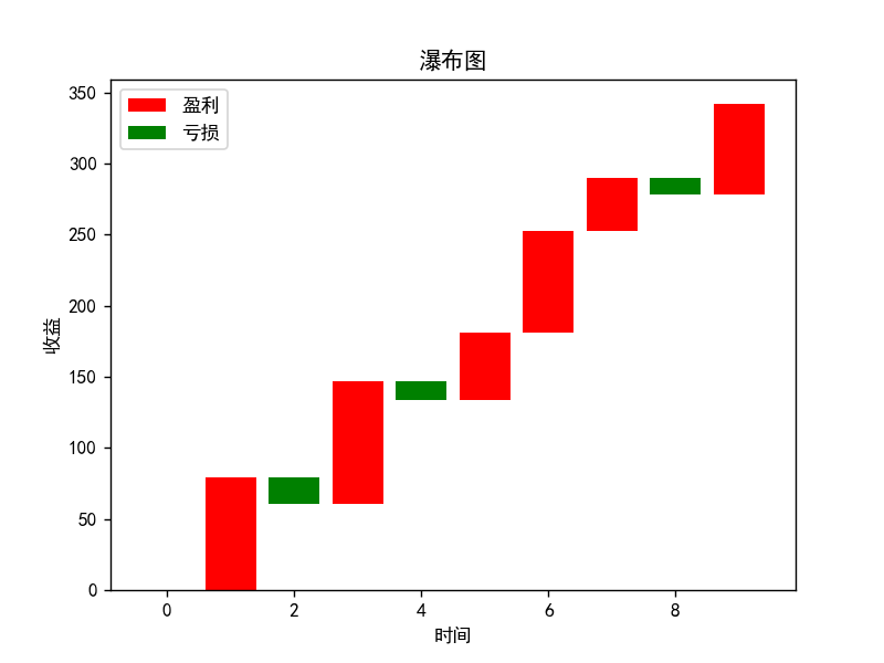
瀑布图
瀑布图-matplotlib
# 收益瀑布图
import numpy as np
import matplotlib.pyplot as plt
import random

plt.rcParams['font.sans-serif'] = ['SimHei']  # 解决中文乱码问题
plt.rcParams['axes.unicode_minus'] = False  # 正常显示负号
profit = [random.randint(-50, 100) for i in range(10)]
bottom = 0
bar_width = 0.8
x_tic = np.arange(len(profit), dtype=np.float64)
for i in range(10):
    x = x_tic[i]
    y = profit[i]
    if profit[i] > 0:
        label1 = '盈利'
        revenue = plt.bar(x, y, bar_width, align='center', bottom=bottom, label=label1, color='red')
    else:
        label1 = '亏损'
        cost = plt.bar(x, y, bar_width, align='center', bottom=bottom, label=label1, color='green')
    bottom += y
    x += 0.8

plt.legend(handles=[revenue, cost])
plt.title("瀑布图")
plt.xlabel('时间')
plt.ylabel('收益')
plt.show()
瀑布图-pyecharts
参考:使用 Pyecharts 制作 Bar(柱状图/条形图/瀑布图)
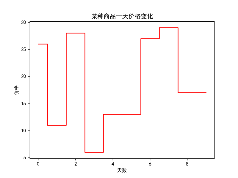
步进图
步进图1-
# 步近图
import matplotlib.pyplot as plt
import random

plt.rcParams['font.sans-serif'] = ['SimHei']  # 解决中文乱码问题
y = [random.randint(0, 30) for i in range(10)]
x = [i for i in range(10)]
plt.plot(x, y, drawstyle='steps-mid', c='red')
plt.xlabel('天数')
plt.ylabel('价格')
plt.title('某种商品十天价格变化')
plt.show()
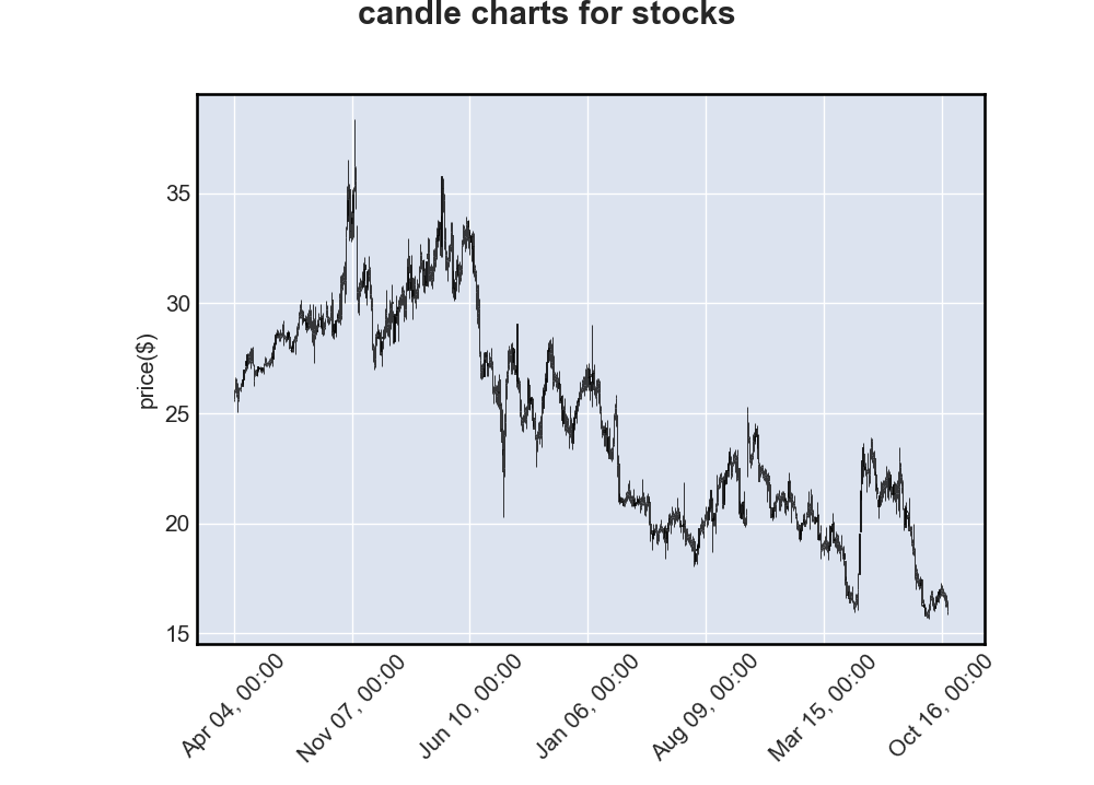
烛形图-
# 烛形图
import tushare as ts
import mplfinance as mpf
import pandas as pd

# 获得数据
quotes = ts.get_hist_data('603970', '2020')
print(quotes.head())
# 将索引转化为需要的格式
quotes.index = pd.to_datetime(quotes.index)
mpf.plot(quotes, type="candle", title="candle charts for stocks", ylabel="price($)")
教材截图