目录
完整文件下载地址:resnet 基于迁移学习对 CIFAR10 数据集的分类
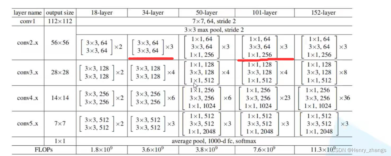
1. resnet 网络
Resnet 网络的搭建:
import torch
import torch.nn as nn


# residual block
class BasicBlock(nn.Module):
    expansion = 1

    def __init__(self,in_channel,out_channel,stride=1,downsample=None):
        super(BasicBlock,self).__init__()
        self.conv1 = nn.Conv2d(in_channel,out_channel,kernel_size=3,stride=stride,padding=1,bias=False) # 第一层的话,可能会缩小size,这时候 stride = 2
        self.bn1 = nn.BatchNorm2d(out_channel)
        self.relu = nn.ReLU()

        self.conv2 = nn.Conv2d(out_channel,out_channel,kernel_size=3,stride=1,padding=1,bias=False)
        self.bn2 = nn.BatchNorm2d(out_channel)
        self.downsample = downsample

    def forward(self,x):
        identity = x
        if self.downsample is not None:     # 有下采样,意味着需要1*1进行降维,同时channel翻倍,residual block虚线部分
            identity = self.downsample(x)

        out = self.conv1(x)
        out = self.bn1(out)
        out = self.relu(out)

        out = self.conv2(out)
        out = self.bn2(out)

        out += identity
        out = self.relu(out)

        return out


# bottleneck
class Bottleneck(nn.Module):
    expansion = 4       # 卷积核的变化

    def __init__(self,in_channel,out_channel,stride=1,downsample=None):
        super(Bottleneck,self).__init__()
        # 1*1 降维度 --------> padding默认为 0,size不变,channel被降低
        self.conv1 = nn.Conv2d(in_channel,out_channel,kernel_size=1,stride=1,bias=False)
        self.bn1 = nn.BatchNorm2d(out_channel)
        # 3*3 卷积
        self.conv2 = nn.Conv2d(out_channel,out_channel,kernel_size=3,stride=stride,bias=False)
        self.bn2 = nn.BatchNorm2d(out_channel)
        # 1*1 还原维度 --------> padding默认为 0,size不变,channel被还原
        self.conv3 = nn.Conv2d(out_channel,out_channel*self.expansion,kernel_size=1,stride=1,bias=False)
        self.bn3 = nn.BatchNorm2d(out_channel*self.expansion)
        # other
        self.relu = nn.ReLU(inplace=True)
        self.downsample =downsample

    def forward(self,x):
        identity = x
        if self.downsample is not None:
            identity = self.downsample(x)

        out = self.conv1(x)
        out = self.bn1(out)
        out = self.relu(out)

        out = self.conv2(out)
        out = self.bn2(out)
        out = self.relu(out)

        out = self.conv3(out)
        out = self.bn3(out)

        out += identity
        out = self.relu(out)

        return out


# resnet
class ResNet(nn.Module):
    def __init__(self,block,block_num,num_classes=1000,include_top=True):
        super(ResNet, self).__init__()
        self.include_top = include_top
        self.in_channel = 64        # max pool 之后的 depth
        # 网络最开始的部分,输入是RGB图像,经过卷积,图像size减半,通道变为64
        self.conv1 = nn.Conv2d(3,self.in_channel,kernel_size=7,stride=2,padding=3,bias=False)
        self.bn1 = nn.BatchNorm2d(self.in_channel)
        self.relu = nn.ReLU(inplace=True)
        self.maxpool = nn.MaxPool2d(kernel_size=3,stride=2,padding=1)   # size减半,padding = 1

        self.layer1 = self.__make_layer(block,64,block_num[0])                # conv2_x
        self.layer2 = self.__make_layer(block,128,block_num[1],stride=2)      # conv3_x
        self.layer3 = self.__make_layer(block,256,block_num[2],stride=2)      # conv4_X
        self.layer4 = self.__make_layer(block,512,block_num[3],stride=2)      # conv5_x

        if self.include_top:    # 分类部分
            self.avgpool = nn.AdaptiveAvgPool2d((1,1))      # out_size = 1*1
            self.fc = nn.Linear(512*block.expansion,num_classes)

    def __make_layer(self,block,channel,block_num,stride=1):
        downsample =None
        if stride != 1 or self.in_channel != channel*block.expansion:     # shortcut 部分,1*1 进行升维
            downsample=nn.Sequential(
                nn.Conv2d(self.in_channel,channel*block.expansion,kernel_size=1,stride=stride,bias=False),
                nn.BatchNorm2d(channel*block.expansion)
            )

        layers =[]
        layers.append(block(self.in_channel, channel, downsample =downsample, stride=stride))
        self.in_channel = channel * block.expansion

        for _ in range(1,block_num):    # residual 实线的部分
            layers.append(block(self.in_channel,channel))

        return nn.Sequential(*layers)

    def forward(self,x):
        # resnet 前面的卷积部分
        x = self.conv1(x)
        x = self.bn1(x)
        x = self.relu(x)
        x = self.maxpool(x)
        # residual 特征提取层
        x = self.layer1(x)
        x = self.layer2(x)
        x = self.layer3(x)
        x = self.layer4(x)
        # 分类
        if self.include_top:
            x = self.avgpool(x)
            x = torch.flatten(x,start_dim=1)
            x = self.fc(x)

        return x


# 定义网络
def resnet34(num_classes=1000,include_top=True):
    return ResNet(BasicBlock,[3,4,6,3],num_classes=num_classes,include_top=include_top)


def resnet101(num_classes=1000,include_top=True):
    return ResNet(Bottleneck,[3,4,23,3],num_classes=num_classes,include_top=include_top)
这里自定义了resnet34和resnet101网络,区别是更deep的网络,参数会非常多,所以这里对于更深网络的残差块,用1*1卷积进行了降维(bottleneck模块)

2. 迁移学习-train
这里用了官方提供了预训练权重
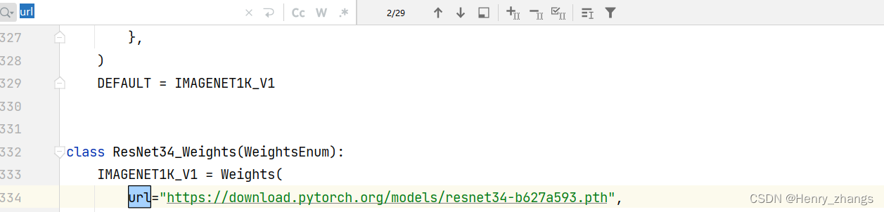
2.1 下载预训练权重
首先导入官方定义的模型:
import torchvision.models.resnet然后进入resnet就行了,就可以看到。找不到的话,可以搜索一下 url
这里用的是resnet34 对CIFAR10分类
2.2 训练过程
迁移学习的时候,要遵循预处理方式
加载预训练权重:
关于迁移学习更为具体的不再本章介绍,后面会单独再写
# 构建网络
net = resnet34()        # 不需要设定参数
pre_model = './resnet_pre_model.pth'        # 预训练权重
missing_keys,unexpected_keys = net.load_state_dict(torch.load((pre_model)),strict=False)
in_channel = net.fc.in_features         # fc
net.fc = nn.Linear(in_channel,10)       # 将最后全连接层改变
net.to(DEVICE)
这里实例化网络的时候,要按照预训练权重的网络分类1000,加载好权重的时候。找到网络的最后一层,更改为新的全连接层就行
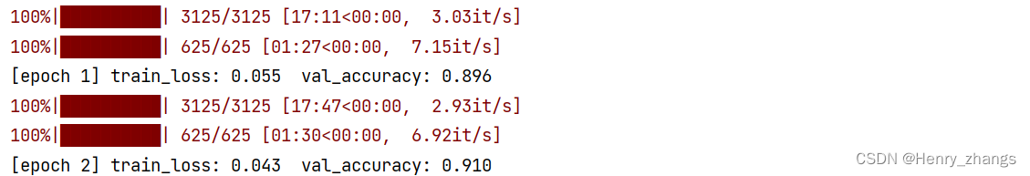
2.3 训练损失+正确率
这里训练的过程较慢,训练了两个epoch就手动停止了
2.4 代码
import torch
import torch.nn as nn
from torchvision import transforms, datasets
import torch.optim as optim
from model import resnet34
from torch.utils.data import DataLoader
from tqdm import tqdm
DEVICE = 'cuda' if torch.cuda.is_available() else 'cpu'
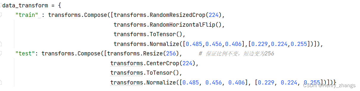
data_transform = {
"train" : transforms.Compose([transforms.RandomResizedCrop(224),
transforms.RandomHorizontalFlip(),
transforms.ToTensor(),
transforms.Normalize([0.485,0.456,0.406],[0.229,0.224,0.255])]),
"test": transforms.Compose([transforms.Resize(256), # 保证比例不变,短边变为256
transforms.CenterCrop(224),
transforms.ToTensor(),
transforms.Normalize([0.485, 0.456, 0.406], [0.229, 0.224, 0.255])])}
# 训练集
trainset = datasets.CIFAR10(root='./data', train=True, download=False, transform=data_transform['train'])
trainloader = DataLoader(trainset, batch_size=16, shuffle=True)
# 测试集
testset = datasets.CIFAR10(root='./data', train=False, download=False, transform=data_transform['test'])
testloader = DataLoader(testset, batch_size=16, shuffle=False)
# 样本的个数
num_trainset = len(trainset) # 50000
num_testset = len(testset) # 10000
# 构建网络
net = resnet34() # 不需要设定参数
pre_model = './resnet_pre_model.pth' # 预训练权重
missing_keys,unexpected_keys = net.load_state_dict(torch.load((pre_model)),strict=False)
in_channel = net.fc.in_features # fc
net.fc = nn.Linear(in_channel,10) # 将最后全连接层改变
net.to(DEVICE)
# 加载损失和优化器
loss_function = nn.CrossEntropyLoss()
optimizer = optim.Adam(net.parameters(), lr=0.0001)
best_acc = 0.0
save_path = './resnet.pth'
for epoch in range(5):
net.train() # 训练模式
running_loss = 0.0
for data in tqdm(trainloader):
images, labels = data
images, labels = images.to(DEVICE), labels.to(DEVICE)
optimizer.zero_grad()
out = net(images) # 总共有三个输出
loss = loss_function(out,labels)
loss.backward() # 反向传播
optimizer.step()
running_loss += loss.item()
# test
net.eval() # 测试模式
acc = 0.0
with torch.no_grad():
for test_data in tqdm(testloader):
test_images, test_labels = test_data
test_images, test_labels = test_images.to(DEVICE), test_labels.to(DEVICE)
outputs = net(test_images)
predict_y = torch.max(outputs, dim=1)[1]
acc += (predict_y == test_labels).sum().item()
accurate = acc / num_testset
train_loss = running_loss / num_trainset
print('[epoch %d] train_loss: %.3f test_accuracy: %.3f' %
(epoch + 1, train_loss, accurate))
if accurate > best_acc:
best_acc = accurate
torch.save(net.state_dict(), save_path)
print('Finished Training')
3. resnet 在 CIFAR10 的预测
展示的结果为:
代码:
import os
os.environ['KMP_DUPLICATE_LIB_OK'] = 'True'
import torch
import numpy as np
import matplotlib.pyplot as plt
from model import resnet34
from torchvision.transforms import transforms
from torch.utils.data import DataLoader
import torchvision
classes = ('plane', 'car', 'bird', 'cat', 'deer', 'dog', 'frog', 'horse', 'ship', 'truck')
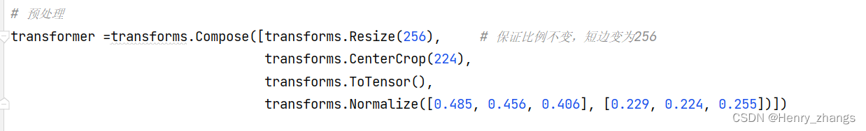
# 预处理
transformer =transforms.Compose([transforms.Resize(256), # 保证比例不变,短边变为256
transforms.CenterCrop(224),
transforms.ToTensor(),
transforms.Normalize([0.485, 0.456, 0.406], [0.229, 0.224, 0.255])])
# 加载模型
DEVICE = 'cuda' if torch.cuda.is_available() else 'cpu'
model = resnet34(num_classes=10)
model.load_state_dict(torch.load('./resnet.pth'))
model.to(DEVICE)
# 加载数据
testSet = torchvision.datasets.CIFAR10(root='./data', train=False, download=False, transform=transformer)
testLoader = DataLoader(testSet, batch_size=12, shuffle=True)
# 获取一批数据
imgs, labels = next(iter(testLoader))
imgs = imgs.to(DEVICE)
# show
with torch.no_grad():
model.eval()
prediction = model(imgs) # 预测
prediction = torch.max(prediction, dim=1)[1]
prediction = prediction.data.cpu().numpy()
plt.figure(figsize=(12, 8))
for i, (img, label) in enumerate(zip(imgs, labels)):
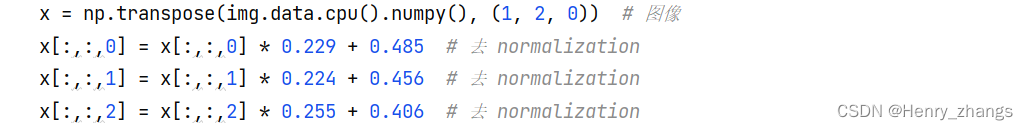
x = np.transpose(img.data.cpu().numpy(), (1, 2, 0)) # 图像
x[:,:,0] = x[:,:,0] * 0.229 + 0.485 # 去 normalization
x[:,:,1] = x[:,:,1] * 0.224 + 0.456 # 去 normalization
x[:,:,2] = x[:,:,2] * 0.255 + 0.406 # 去 normalization
y = label.numpy().item() # label
plt.subplot(3, 4, i + 1)
plt.axis(False)
plt.imshow(x)
plt.title('R:{},P:{}'.format(classes[y], classes[prediction[i]]))
plt.show()预处理:
加载模型:这里可以之间设置分类是10

展示:这里反归一化的时候,要经过下面的变换