face3d: Python tools for processing 3D face
git code: https://github.com/yfeng95/face3d
paper list: PaperWithCode
3DMM方法,基于平均人脸模型,可实现线性的人脸生成。此外,基于人脸关键点,还能渲染对应的三维人脸模型。
目录
- face3d: Python tools for processing 3D face
- 一、BFM(Basel Face Model)介绍
-
- 1.1 3DMM模型的定义
- 1.2 3dmm例子解读
-
- 1.2.0 加载相关库
- 1.2.1 加载BFM模型
- 1.2.2 生成人脸网格:顶点(表示形状)和颜色(表示纹理)
- 1.2.3 网格位置变换
- 1.2.4 将3D对象(网格数据)渲染为2D图像
- 2.1 目标估计
- 2.2 2D和3D特征点之间的转化
- 2.3 最小能量方程
- 3.1 反向过程代码解读
- 通过fit.fit_points函数来拆分讲解
- 2.4 参数估计 s , R , t 2 d s, R, t_{2d} s,R,t2d
- 2.4.1 黄金标准算法
- 总结
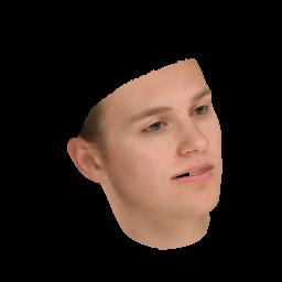
基于3DMM模型的生成1:正常

基于3DMM模型的生成2:微笑
3DMM模型的原理是怎样的?如何实现二维与三维的生成呢?
要回答上述问题,必须要弄清楚3DMM提供了哪些信息?如何操控这些信息以实现特定的人脸生成。
文中部分图片来自:Face3D学习笔记
一、BFM(Basel Face Model)介绍
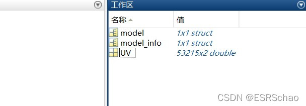
在系列一中介绍了使用generate.m文件来产生BFM模型,它具体包含BFM.mat,BFM_info.mat,BFM_UV.mat等数据。
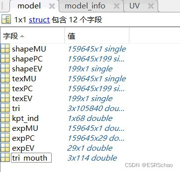
BFM.mat数据格式
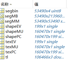
BFM_info.mat格式

BFM_UV格式
这些.mat文件中包含的信息具有什么含义呢?下面从原理方面进行如下解析:
1.1 3DMM模型的定义
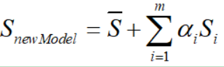
3DMM有如下公式:

其中:
- Z ^ \hat{Z} Z^表示平均人脸形状
- S i S_i Si表示形状PCA主成分
- α i \alpha_i αi表示形状系数
- E i E_i Ei表示人脸表情PCA主成分
- β i \beta_i βi表示人脸表情系数
BFM模型不提供原始人脸数据或参数化后的人脸,只提供形状和纹理信息。在BFM模型经过去中心化的数据所对应的m、n均为199。
01_MorphableModel.mat数据格式
如下表所示:
| 名称 | 含义 | 维度 |
|---|---|---|
| shapeMU | 平均人脸形状 | (160470,1) |
| shapePC | 形状主成分 | (160470,199) |
| shapeEV | 形状主成分方差 | (199,1) |
| texMU | 平均人脸纹理 | (160470,1) |
| texPC | 纹理主成分 | (160470,199) |
| texEV | 纹理主成分方差 | (199,1) |
| tl | 三角面片 | (106466,3) |
| segbin | 区域分割信息 | (53490,4) |
1.2 3dmm例子解读
3dmm例子实现的两个任务:
- 正向过程:基于BFM模型,给定3dmm参数,生产mesh数据和对应的人脸数据
- 反向过程:即拟合,如果假设有人脸的关键点信息,根据BFM模型如何生成对应的三维人脸。
1.2.0 加载相关库
''' 3d morphable model example
3dmm parameters --> mesh
fitting: 2d image + 3dmm -> 3d face
'''
import os, sys
import subprocess
import numpy as np
import scipy.io as sio
from skimage import io
from time import time
import matplotlib.pyplot as plt

sys.path.append('..')
import face3d
from face3d import mesh
from face3d.morphable_model import MorphabelModel
1.2.1 加载BFM模型
# --------------------- Forward: parameters(shape, expression, pose) --> 3D obj --> 2D image  ---------------
# --- 1. load model
bfm = MorphabelModel('Data/BFM/Out/BFM.mat')
print('init bfm model success')
其中,MorphabelModel所对应的源码为
class  MorphabelModel(object):
    """docstring for  MorphabelModel
    model: nver: number of vertices. ntri: number of triangles. *: must have. ~: can generate ones array for place holder.
            'shapeMU': [3*nver, 1]. *
            'shapePC': [3*nver, n_shape_para]. *
            'shapeEV': [n_shape_para, 1]. ~
            'expMU': [3*nver, 1]. ~
            'expPC': [3*nver, n_exp_para]. ~
            'expEV': [n_exp_para, 1]. ~
            'texMU': [3*nver, 1]. ~
            'texPC': [3*nver, n_tex_para]. ~
            'texEV': [n_tex_para, 1]. ~
            'tri': [ntri, 3] (start from 1, should sub 1 in python and c++). *
            'tri_mouth': [114, 3] (start from 1, as a supplement to mouth triangles). ~
            'kpt_ind': [68,] (start from 1). ~
    """
    def __init__(self, model_path, model_type = 'BFM'):
        super( MorphabelModel, self).__init__()
        if model_type=='BFM':
            self.model = load.load_BFM(model_path)
        else:
            print('sorry, not support other 3DMM model now')
            exit()

        # fixed attributes
        self.nver = self.model['shapePC'].shape[0]/3
        self.ntri = self.model['tri'].shape[0]
        self.n_shape_para = self.model['shapePC'].shape[1]
        self.n_exp_para = self.model['expPC'].shape[1]
        self.n_tex_para = self.model['texPC'].shape[1]

        self.kpt_ind = self.model['kpt_ind']
        self.triangles = self.model
['tri']
        self.full_triangles = np.vstack((self.model['tri'], self.model['tri_mouth']))
其中,self.model = load.load_BFM(model_path)所读取的model包含的信息如下表所示:

| 名称 | 含义 | 格式 |
|---|---|---|
| shapeMU | 平均人脸形状 | (159645,1) |
| shapePC | 形状主成分 | (159645,199) |
| shapeEV | 形状主成分方差 | (199,1) |
| expMU | 平均人脸表情 | (159645,1) |
| expPC | 表情主成分 | (159645,29) |
| expEV | 表情主成分方差 | (29,1) |
| texMU | 平均人脸纹理 | (159645,1) |
| texPC | 纹理主成分 | (159645,199) |
| texEV | 纹理主成分方差 | (199,1) |
| tri | 三角格坐标 | (105840,3) |
| tri_mouth | 嘴部三角格坐标 | (114,3) |
| kpt_ind | 特征点 | (68,) |
1.2.2 生成人脸网格:顶点(表示形状)和颜色(表示纹理)
这里采用随机的形状系数和表情系数来生成人脸
# --- 2. generate face mesh: vertices(represent shape) & colors(represent texture)
sp = bfm.get_shape_para('random')
ep = bfm.get_exp_para('random')
vertices = bfm.generate_vertices(sp, ep)

tp = bfm.get_tex_para('random')
colors = bfm.generate_colors(tp)
colors = np.minimum(np.maximum(colors, 0), 1)
sp对应形状系数 α \alpha α,ep对应表情系数 β \beta β, t p tp tp对应的是纹理系数。这些系数均随机产生。其中调用函数定义如下:
	def get_shape_para(self, type = 'random'):
        if type == 'zero':
            sp = np.zeros((self.n_shape_para, 1))
        elif type == 'random':
            sp = np.random.rand(self.n_shape_para, 1)*1e04
        return sp

    def get_exp_para(self, type = 'random'):
        if type == 'zero':
            ep = np.zeros((self.n_exp_para, 1))
        elif type == 'random':
            ep = -1.5 + 3*np.random.random([self.n_exp_para, 1])
            ep[6:, 0] = 0

        return ep

    def generate_vertices(self, shape_para, exp_para):
        '''
        Args:
            shape_para: (n_shape_para, 1)
            exp_para: (n_exp_para, 1)
        Returns:
            vertices: (nver, 3)
        '''
        vertices = self.model['shapeMU'] + \
                   self.model['shapePC'].dot(shape_para) + \
                   self.model['expPC'].dot(exp_para)
        vertices = np.reshape(vertices, [int(3), int(len(vertices)/3)], 'F').T

        return vertices

    # -------------------------------------- texture: here represented with rgb value(colors) in vertices.
    def get_tex_para(self, type = 'random'):
        if type == 'zero':
            tp = np.zeros((self.n_tex_para, 1))
        elif type == 'random':
            tp = np.random.rand(self.n_tex_para, 1)
        return tp

    def generate_colors(self, tex_para):
        '''
        Args:
            tex_para: (n_tex_para, 1)
        Returns:
            colors: (nver, 3)
        '''
        colors = self.model['texMU'] + self.model['texPC'].dot(tex_para)
        colors = np.reshape(colors, [int(3), int(len(colors)/3)], 'F').T/255.

        return colors
不难发现,generate_vertices产生顶点的函数,主要使用shape和expression信息。纹理部分也采用类似原理计算。到此,新的人脸模型产生。

这里通过改变$\alpha$和$\beta$系数,可以生成不同表情和形状的人脸,如开头展示的两组人脸就是采用不同系数而产生的。
1.2.3 网格位置变换
该部分在上一期的系列中介绍过,再给定尺度、旋转角度和平移坐标的信息后,即可得到变换后的位置。
# --- 3. transform vertices to proper position
s = 8e-04
angles = [10, 30, 20]
t = [0, 0, 0]
transformed_vertices = bfm.transform(vertices, s, angles, t)
projected_vertices = transformed_vertices.copy() # using stantard camera & orth projection
1.2.4 将3D对象(网格数据)渲染为2D图像
同上一期的pipeline相似,给定生成图像的宽高,可以将生产的3D网格转化为平面图。
# --- 4. render(3d obj --> 2d image)
# set prop of rendering
h = w = 256; c = 3
image_vertices = mesh.transform.to_image(projected_vertices, h, w)
image = mesh.render.render_colors(image_vertices, bfm.triangles, colors, h, w)
#可使用如下代码将渲染后的二维图像可视化
plt.imshow(image)
plt.show()
以上部分实现的前向过程,即给出参数(形状,表情,纹理),生产三维对象,再转化为平面图。
Forward: parameters(shape, expression, pose) --> 3D obj --> 2D image
反向过程
参考:https://blog.csdn.net/likewind1993/article/details/81455882
反向过程,指的是给定人脸关键点的信息,如何生产对应的三维人脸模型。
通过3DMM的定义可知,要想生成特定的人脸,必须要知道shape和expression系数等。如果不能直接的给出这些参数,但是能够知道人脸关键点的位置,能够通过人脸位置之间的映射关系,找到参数的求解呢?这里借助源码来充分理解。
2.1 目标估计
3DMM最早出现于99年的一篇文章:https://blog.csdn.net/likewind1993/article/details/79177566,论文里提出了一种人脸的线性表示方法。该方法可以通过以下实现:
(原文中还加入了纹理部分,但是拟合效果不够好,一般直接从照片中提取纹理进行贴合,因此这里只给出重建人脸形状的部分)。
在2014年, FacewareHouse论文基于3DMM模型公开了一个人脸表情数据库,使得3DMM更加发扬光大,其将人脸模型的线性表示扩展为:

即在原来的基础上加入了Expression表情信息。
于是,人脸重建问题转为了求解 α \alpha α和 β \beta β系数的问题。
2.2 2D和3D特征点之间的转化
假设一张人脸照片,首先利用人脸对齐算法计算得到目标二维人脸的68个特征点坐标 X X X,在BFM模型中有对应的68个特征点 X 3 d X_{3d} X3d,根据这些信息便可求出 α \alpha α和 β \beta β系数,将平均人脸模型与照片中的脸部进行拟合。投影后忽略第三维,其特征点之间的对应关系如下:
因此,可以将BFM中的三维人脸关键点投影到二维平面,即:
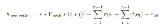
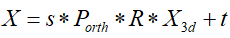
其中, X p r o j e c t i o n X_{projection} Xprojection是三维映射到二维平面的点, P o r t h P_{orth} Porth=[[1,0,0],[0,1,0]]为正交投影矩阵,R(3,3)为旋转矩阵, t 2 d t_{2d} t2d为位移矩阵。
2.3 最小能量方程
该问题可以转化为求解满足以下能量方程的系数( s , R , t 2 d , α , β s, R, t_{2d}, \alpha, \beta s,R,t2d,α,β)
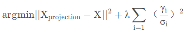
这里加入了正则化项,其中 γ \gamma γ 是PCA系数(包含形状系数 α \alpha α和表情系数 β \beta β), σ \sigma σ表示对应的主成分偏差。
即,由上式求解可以使得三维模型中的68特征点投影到二维平面上的值与二维平面原68个特征点距离相差最小。
那么,如何详细的求解呢?
我们需要求得的参数主要有 s , R , t 2 d , α , β s, R, t_{2d}, \alpha, \beta s,R,t2d,α,β,这里可以把参数分为三个部分, s , R , t 2 d s, R, t_{2d} s,R,t2d, α \alpha α和 β \beta β
求解算法如下:
- 将α以及β初始化为0
- 求出 s , R , t 2 d s, R, t_{2d} s,R,t2d
- 将上一步求出的 s , R , t 2 d s, R, t_{2d} s,R,t2d代入,求出α
- 将之前求出的 s , R , t 2 d s, R, t_{2d} s,R,t2d以及α代入,求出β
- 利用求得的α以及β,重复2-4步骤进行迭代
3.1 反向过程代码解读
# -------------------- Back:  2D image points and corresponding 3D vertex indices-->  parameters(pose, shape, expression) ------
## only use 68 key points to fit
x = projected_vertices[bfm.kpt_ind, :2] # 2d keypoint, which can be detected from image
X_ind = bfm.kpt_ind # index of keypoints in 3DMM. fixed.

# fit
fitted_sp, fitted_ep, fitted_s, fitted_angles, fitted_t = bfm.fit(x, X_ind, max_iter = 3)

# verify fitted parameters
fitted_vertices = bfm.generate_vertices(fitted_sp, fitted_ep)
transformed_vertices = bfm.transform(fitted_vertices, fitted_s, fitted_angles, fitted_t)

image_vertices = mesh.transform.to_image(transformed_vertices, h, w)
fitted_image = mesh.render.render_colors(image_vertices, bfm.triangles, colors, h, w)
其中,x就是公式中的二维特征点X,这里给出的二维特征点来自于BFM。 X i n d X_{ind} Xind是BFM模型三维特征点的索引,并非坐标。
然后执行拟合部分:
fitted_sp, fitted_ep, fitted_s, fitted_angles, fitted_t = bfm.fit(x, X_ind, max_iter = 3
bfm.fit的定义如下:
def fit(self, x, X_ind, max_iter = 4, isShow = False):
        ''' fit 3dmm & pose parameters
        Args:
            x: (n, 2) image points
            X_ind: (n,) corresponding Model vertex indices
            max_iter: iteration
            isShow: whether to reserve middle results for show
        Returns:
            fitted_sp: (n_sp, 1). shape parameters
            fitted_ep: (n_ep, 1). exp parameters
            s, angles, t
        '''
        if isShow:
            fitted_sp, fitted_ep, s, R, t = fit.fit_points_for_show(x, X_ind, self.model, n_sp = self.n_shape_para, n_ep = self.n_exp_para, max_iter = max_iter)
            angles = np.zeros((R.shape[0], 3))
            for i in range(R.shape[0]):
                angles[i] = mesh.transform.matrix2angle(R[i])
        else:
            fitted_sp, fitted_ep, s, R, t = fit.fit_points(x, X_ind, self.model, n_sp = self.n_shape_para, n_ep = self.n_exp_para, max_iter = max_iter)
            angles = mesh.transform.matrix2angle(R)
        return fitted_sp, fitted_ep, s, angles, t
这里执行了fit_points和matrix2angle函数,其定义分别有:
def fit_points(x, X_ind, model, n_sp, n_ep, max_iter = 4):
    '''
    Args:
        x: (n, 2) image points
        X_ind: (n,) corresponding Model vertex indices
        model: 3DMM
        max_iter: iteration
    Returns:
        sp: (n_sp, 1). shape parameters
        ep: (n_ep, 1). exp parameters
        s, R, t
    '''
    x = x.copy().T

    #-- init
    sp = np.zeros((n_sp, 1), dtype = np.float32)
    ep = np.zeros((n_ep, 1), dtype = np.float32)

    #-------------------- estimate
    X_ind_all = np.tile(X_ind[np.newaxis, :], [3, 1])*3
    X_ind_all[1, :] += 1
    X_ind_all[2, :] += 2
    valid_ind = X_ind_all.flatten('F')

    shapeMU = model['shapeMU'][valid_ind, :]
    shapePC = model['shapePC'][valid_ind, :n_sp]
    expPC = model['expPC'][valid_ind, :n_ep]

    for i in range(max_iter):
        X = shapeMU + shapePC.dot(sp) + expPC.dot(ep)
        X = np.reshape(X, [int(len(X)/3), 3]).T

        #----- estimate pose
        P = mesh.transform.estimate_affine_matrix_3d22d(X.T, x.T)
        s, R, t = mesh.transform.P2sRt(P)
        rx, ry, rz = mesh.transform.matrix2angle(R)
        # print('Iter:{}; estimated pose: s {}, rx {}, ry {}, rz {}, t1 {}, t2 {}'.format(i, s, rx, ry, rz, t[0], t[1]))

        #----- estimate shape
        # expression
        shape = shapePC.dot(sp)
        shape = np.reshape(shape, [int(len(shape)/3), 3]).T
        ep = estimate_expression(x, shapeMU, expPC, model['expEV'][:n_ep,:], shape, s, R, t[:2], lamb = 0.002)

        # shape
        expression = expPC.dot(ep)
        expression = np.reshape(expression, [int(len(expression)/3), 3]).T
        sp = estimate_shape(x, shapeMU, shapePC, model['shapeEV'][:n_sp,:], expression, s, R, t[:2], lamb = 0.004)

    return sp, ep, s, R, t
通过fit.fit_points函数来拆分讲解
(1)初始化α , β为0
x = x.copy().T
    #-- init
    sp = np.zeros((n_sp, 1), dtype = np.float32)
    ep = np.zeros((n_ep, 1), dtype = np.float32)
x取转置,格式变为(2,68)
sp即α,ep即β。将它们赋值为格式(199,1)的零向量。
X 3 d X_{3d} X3d进行坐标转换
由于BFM模型中的顶点坐标储存格式为 x 1 , y 1 , z 1 , x 2 , y 2 , z 2 , . . . {x_1,y_1,z_1,x_2,y_2,z_2,...} x1,y1,z1,x2,y2,z2,...
而在X_ind中只给出了三位特征点坐标的位置,所以应该根据X_ind获取 X 3 d X_{3d} X3d的XYZ坐标数据。
X_ind_all = np.tile(X_ind[np.newaxis, :], [3, 1])*3
    X_ind_all[1, :] += 1
    X_ind_all[2, :] += 2
    valid_ind = X_ind_all.flatten('F')
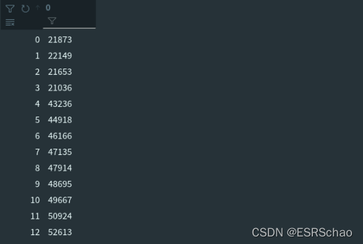
X_ind数据如下,是一个(68,1)的位置数据。
X_ind_all = np.tile(X_ind[np.newaxis, :], [3, 1])*3
X_ind_all拓展为(3,68)并乘3来定位到坐标位置:
X_ind_all[1, :] += 1
X_ind_all[2, :] += 2
再将第二行加一、第三行加二来对于Y坐标和Z坐标。
然后将它们拉伸为一维数组。flatten适用于numpy对应即array和mat,list不适用。
valid_ind = X_ind_all.flatten('F')
'F’表示以列优先展开。
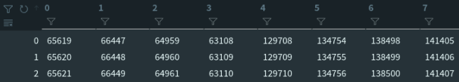
合并后的结果valid_ind如下图:
通过合并后的valid_ind得到对应特征点的人脸形状、形状主成分、表情主成分这三种数据。
shapeMU = model['shapeMU'][valid_ind, :]
shapePC = model['shapePC'][valid_ind, :n_sp]
expPC = model['expPC'][valid_ind, :n_ep]
人脸形状shapeMU数据格式(683,1)
形状主成分shapePC数据格式(683,199)
表情主成分expPC数据格式(68*3,29)
for i in range(max_iter):
        X = shapeMU + shapePC.dot(sp) + expPC.dot(ep)
        X = np.reshape(X, [int(len(X)/3), 3]).T

        #----- estimate pose
        P = mesh.transform.estimate_affine_matrix_3d22d(X.T, x.T)
        s, R, t = mesh.transform.P2sRt(P)
        rx, ry, rz = mesh.transform.matrix2angle(R)
        # print('Iter:{}; estimated pose: s {}, rx {}, ry {}, rz {}, t1 {}, t2 {}'.format(i, s, rx, ry, rz, t[0], t[1]))

        #----- estimate shape
        # expression
        shape = shapePC.dot(sp)
        shape = np.reshape(shape, [int(len(shape)/3), 3]).T
        ep = estimate_expression(x, shapeMU, expPC, model['expEV'][:n_ep,:], shape, s, R, t[:2], lamb = 0.002)

        # shape
        expression = expPC.dot(ep)
        expression = np.reshape(expression, [int(len(expression)/3), 3]).T
        sp = estimate_shape(x, shapeMU, shapePC, model['shapeEV'][:n_sp,:], expression, s, R, t[:2], lamb = 0.004)
    return sp, ep, s, R, t
循环中的max_iter是自行定义的迭代次数,这里的输入为4。
X = shapeMU + shapePC.dot(sp) + expPC.dot(ep)
X = np.reshape(X, [int(len(X)/3), 3]).T
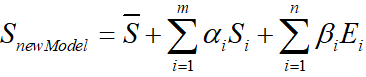
这里的X就是经过如下的运算的 S n e w m o d e l S_{newmodel} Snewmodel,就是新的 X 3 d X_{3d} X3d
真正重点的是mesh.transform.estimate_affine_matrix_3d22d(X.T, x.T),这是网格的拟合部分。
源码如下:
estimate_affine_matrix_3d22d(X, x):
    ''' Using Golden Standard Algorithm for estimating an affine camera
        matrix P from world to image correspondences.
        See Alg.7.2. in MVGCV
        Code Ref: https://github.com/patrikhuber/eos/blob/master/include/eos/fitting/affine_camera_estimation.hpp
        x_homo = X_homo.dot(P_Affine)
    Args:
        X: [n, 3]. corresponding 3d points(fixed)
        x: [n, 2]. n>=4. 2d points(moving). x = PX
    Returns:
        P_Affine: [3, 4]. Affine camera matrix
    '''
    X = X.T; x = x.T
    assert(x.shape[1] == X.shape[1])
    n = x.shape[1]
    assert(n >= 4)

    #--- 1. normalization
    # 2d points
    mean = np.mean(x, 1) # (2,)
    x = x - np.tile(mean[:, np.newaxis], [1, n])
    average_norm = np.mean(np.sqrt(np.sum(x**2, 0)))
    scale = np.sqrt(2) / average_norm
    x = scale * x

    T = np.zeros((3,3), dtype = np.float32)
    T[0, 0] = T[1, 1] = scale
    T[:2, 2] = -mean*scale
    T[2, 2] = 1

    # 3d points
    X_homo = np.vstack((X, np.ones((1, n))))
    mean = np.mean(X, 1) # (3,)
    X = X - np.tile(mean[:, np.newaxis], [1, n])
    m = X_homo[:3,:] - X
    average_norm = np.mean(np.sqrt(np.sum(X**2, 0)))
    scale = np.sqrt(3) / average_norm
    X = scale * X

    U = np.zeros((4,4), dtype = np.float32)
    U[0, 0] = U[1, 1] = U[2, 2] = scale
    U[:3, 3] = -mean*scale
    U[3, 3] = 1

    # --- 2. equations
    A = np.zeros((n*2, 8), dtype = np.float32);
    X_homo = np.vstack((X, np.ones((1, n)))).T
    A[:n, :4] = X_homo
    A[n:, 4:] = X_homo
    b = np.reshape(x, [-1, 1])

    # --- 3. solution
    p_8 = np.linalg.pinv(A).dot(b)
    P = np.zeros((3, 4), dtype = np.float32)
    P[0, :] = p_8[:4, 0]
    P[1, :] = p_8[4:, 0]
    P[-1, -1] = 1

    # --- 4. denormalization
    P_Affine = np.linalg.inv(T).dot(P.dot(U))
    return P_Affine

def P2sRt(P):
    ''' decompositing camera matrix P
    Args:
        P: (3, 4). Affine Camera Matrix.
    Returns:
        s: scale factor.
        R: (3, 3). rotation matrix.
        t: (3,). translation.
    '''
    t = P[:, 3]
    R1 = P[0:1, :3]
    R2 = P[1:2, :3]
    s = (np.linalg.norm(R1) + np.linalg.norm(R2))/2.0
    r1 = R1/np.linalg.norm(R1)
    r2 = R2/np.linalg.norm(R2)
    r3 = np.cross(r1, r2)

    R = np.concatenate((r1, r2, r3), 0)
    return s, R, t
(2)利用黄金标准算法得到一个仿射矩阵 P A P_{A} PA,分解得到 s , R , t 2 d s,R,t_{2d} s,R,t2d
2.4 参数估计 s , R , t 2 d s, R, t_{2d} s,R,t2d
人脸模型中的三维点与对应照片中的二维点存在映射关系,可以用一个3×4的仿射矩阵进行表示。即:
X 2 d = P × X 3 d X_{2d} = P \times X_{3d} X2d=P×X3d
P即是我们需要求的仿射矩阵,作用在三维坐标点上可以得到二维坐标点。
这里使用黄金标准算法(Gold Standard Algorithm)来求该仿射矩阵,estimate_affine_matrix_3d22d部分即黄金标准算法具体过程
2.4.1 黄金标准算法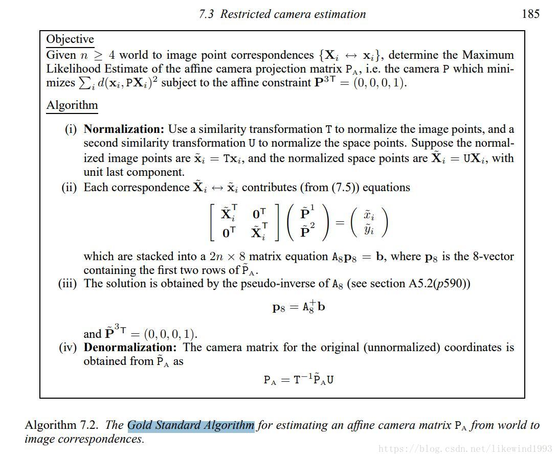
算法表述如下:
目标:在给定多组从3d到2d的图像对应集合(点对的数量>=4),确定仿射相机投影矩阵的最大似然估计。
- 归一化
对二维点 X X X,计算一个相似变换 T T T,使得 X ^ = T X \hat{X}=TX X^=TX,同样的对于三维点 X 3 d X_{3d} X3d,计算 X ^ 3 d = U X 3 d \hat{X}_{3d}=UX_{3d} X^3d=UX3d。
归一化部分的概念在Multiple View Geometry in Computer Vision一书中描述如下:
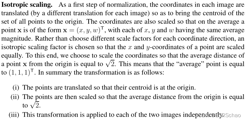
所以归一化可以概述为以下三步:
- 平移所有坐标点,使它们的质心位于原点。
- 然后对这些点进行缩放,使到原点的平均距离等于 2 \sqrt{2} 2 。
- 将该变换应用于图像中的每一幅。
下面结合代码进行讲解:
输入检测,确保输入的二维和三维特征点的数目一致以及特征点数目大于4。
 X = X.T; x = x.T
    assert(x.shape[1] == X.shape[1])
    n = x.shape[1]
    assert(n >= 4)
二维数据归一化:
    #--- 1. normalization
    # 2d points
    mean = np.mean(x, 1) # (2,)
    x = x - np.tile(mean[:, np.newaxis], [1, n])
    average_norm = np.mean(np.sqrt(np.sum(x**2, 0)))
    scale = np.sqrt(2) / average_norm
    x = scale * x

    T = np.zeros((3,3), dtype = np.float32)
    T[0, 0] = T[1, 1] = scale
    T[:2, 2] = -mean*scale
    T[2, 2] = 1
- 平移所有坐标点,使它们的质心位于原点。
经过x=x.T后x的格式变为(2,68)
通过mean = np.mean(x, 1)获取x的X坐标和Y坐标平均值mean,格式为(2,)
这一步x = x - np.tile(mean[:, np.newaxis], [1, n])
x的所有XY坐标都减去刚刚算出的平均值,此时x中的坐标点被平移到了质心位于原点的位置。 - 然后对这些点进行缩放,使到原点的平均距离等于 2 \sqrt{2} 2 。
average_norm = np.mean(np.sqrt(np.sum(x**2, 0)))
算出所有此时所有二维点到原点的平均距离average_norm,这是一个数值。
scale = np.sqrt(2) / average_norm
x = scale * x
算出scale再用scale去乘x坐标,相当与x所有的坐标除以当前的平均距离之后乘以 2 \sqrt{2} 2
这样算出来的所有点到原点的平均距离就被缩放到了$\sqrt{2}¥ - 同时通过计算出的scale和mean可以算出相似变换T
T = np.zeros((3,3), dtype = np.float32)
T[0, 0] = T[1, 1] = scale
T[:2, 2] = -mean*scale
T[2, 2] = 1
# 3d points
    X_homo = np.vstack((X, np.ones((1, n))))
    mean = np.mean(X, 1) # (3,)
    X = X - np.tile(mean[:, np.newaxis], [1, n])
    m = X_homo[:3,:] - X
    average_norm = np.mean(np.sqrt(np.sum(X**2, 0)))
    scale = np.sqrt(3) / average_norm
    X = scale * X

    U = np.zeros((4,4), dtype = np.float32)
    U[0, 0] = U[1, 1] = U[2, 2] = scale
    U[:3, 3] = -mean*scale
    U[3, 3] = 1
三位归一化的原理与二维相似,区别就是所有点到原点的平均距离要被缩放到 3 \sqrt{3} 3 ,以及生成的相似变换矩阵 U U U格式为(4,4)。这不赘述了。
- 对于每组对应点 x i x_i xi~ X i X_i Xi,都有形如 A x = b Ax=b Ax=b 的对应关系存在
# --- 2. equations
    A = np.zeros((n*2, 8), dtype = np.float32);
    X_homo = np.vstack((X, np.ones((1, n)))).T
    A[:n, :4] = X_homo
    A[n:, 4:] = X_homo
    b = np.reshape(x, [-1, 1])
这里结合公式来看,
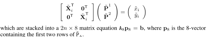
A对应其中的 [ X ^ i T 0 T 0 T X i T ] \begin{bmatrix} \hat{X}^T_i & 0^T\\ 0^T & X^T_i \end{bmatrix} [X^iT0T0TXiT]
b是展开为(68*2,1)格式的x。
求出A的伪逆
 # --- 3. solution
    p_8 = np.linalg.pinv(A).dot(b)
    P = np.zeros((3, 4), dtype = np.float32)
    P[0, :] = p_8[:4, 0]
    P[1, :] = p_8[4:, 0]
    P[-1, -1] = 1
关于A的伪逆的概念和求取方法可以参照Multiple View Geometry in Computer Vision书中的P590以后的内容。这里A的伪逆是利用numpy里面的函数np.linalg.pinv直接计算出来的,非常方便。
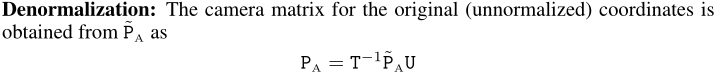
去掉归一化,得到仿射矩阵
 # --- 4. denormalization
    P_Affine = np.linalg.inv(T).dot(P.dot(U))
    return P_Affine
这部分的代码参照公式:
以上四步就是黄金标准算法的完整过程
得到的 P A f f i n e P_{Affine} PAffine就是式中的 P A P_A PA,到这里,我们通过黄金标准算法得到了 X = P A ⋅ X 3 d X = P_A\cdot X_{3d} X=PA⋅X3d中的 P A P_A PA。
将仿射矩阵 P A P_A PA分解得到 s , R , t 2 d s, R, t_{2d} s,R,t2d
s, R, t = mesh.transform.P2sRt(P)
rx, ry, rz = mesh.transform.matrix2angle(R)
其中mesh.transform.P2sRt部分的源码如下:
def P2sRt(P):
    ''' decompositing camera matrix P
    Args:
        P: (3, 4). Affine Camera Matrix.
    Returns:
        s: scale factor.
        R: (3, 3). rotation matrix.
        t: (3,). translation.
    '''
    t = P[:, 3]
    R1 = P[0:1, :3]
    R2 = P[1:2, :3]
    s = (np.linalg.norm(R1) + np.linalg.norm(R2))/2.0
    r1 = R1/np.linalg.norm(R1)
    r2 = R2/np.linalg.norm(R2)
    r3 = np.cross(r1, r2)

    R = np.concatenate((r1, r2, r3), 0)
    return s, R, t
这部分就是将仿射矩阵 R A {R_A} RA (3×4)分解为下图的缩放比例s(1)、旋转矩阵R(3×3)以及平移矩阵t(3×1)。
总结
这里主要介绍基于3DMM模型的前向与反向过程。前向过程,基于3DMM,给出参数的情况下,生产三维对象和二维人脸;反向过程,给出人脸关键点的情况下,估计形状和颜色参数等,形成对应的三维人脸建模。求解α , β 的过程将在下篇文章讲解。