Plotly Express 是一个新的高级 Python 可视化库,它是 Plotly.py 的高级封装,为复杂图表提供简单的语法。最主要的是 Plotly 可以与 Pandas 数据类型 DataFrame 完美的结合,对于数据分析、可视化来说实在是太便捷了,而且是完全免费的,非常值得尝试
下面我们使用 Ployly 的几个内置数据集来进行相关图表绘制的演示
数据集
Plotly 内置的所有数据集都是 DataFrame 格式,也即是与 Pandas 深度契合的体现
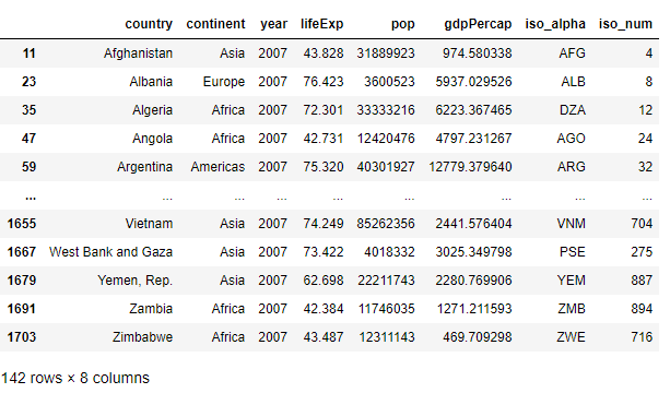
不同国家历年GDP收入与人均寿命
包含字段:国家、洲、年份、平均寿命、人口数量、GDP、国家简称、国家编号
gap = px.data.gapminder()
gap2007 = gap.query("year==2007")
gap2007
Output
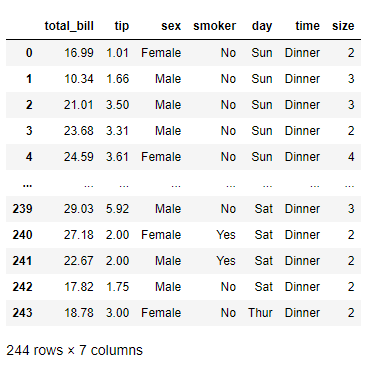
餐馆的订单流水
包含字段:总账单、小费、性别、是否抽烟、星期几、就餐时间、人数
tips = px.data.tips()
tips
Output
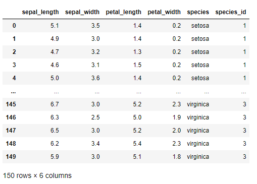
鸢尾花
包含字段:萼片长、萼片宽、花瓣长、花瓣宽、种类、种类编号
iris = px.data.iris()
iris
Output
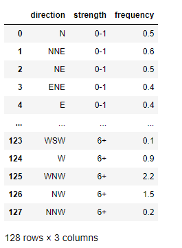
风力
包含字段:方向、强度、数值
wind = px.data.wind()
wind
Output
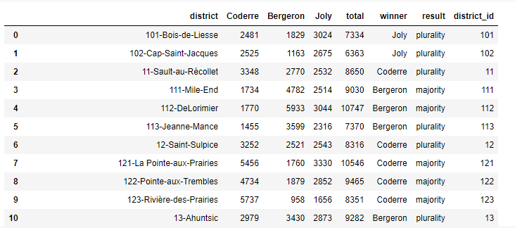
2013年蒙特利尔市长选举投票结果
包括字段:区域、Coderre票数、Bergeron票数、Joly票数、总票数、胜者、结果(占比分类)
election = px.data.election()
election
Output
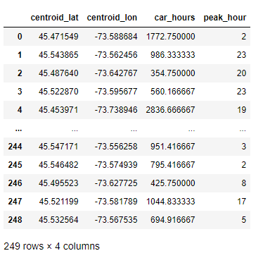
蒙特利尔一个区域中心附近的汽车共享服务的可用性
包括字段:纬度、经度、汽车小时数、高峰小时
carshare = px.data.carshare()
carshare
Output
内置调色面板
Plotly 还用于众多色彩高级的调色板,使得我们在绘制图表的时候不再为颜色搭配烦恼
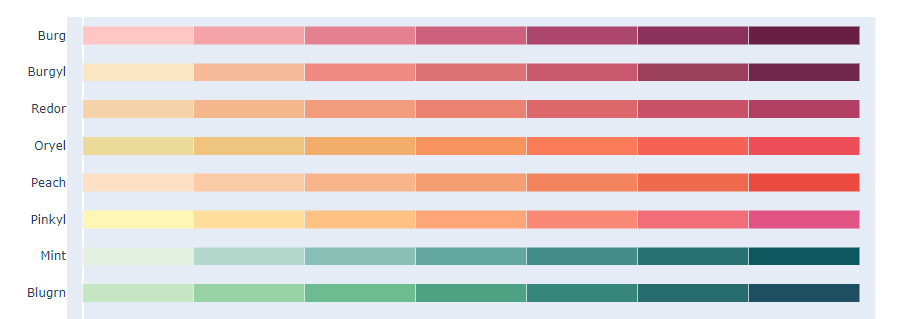
卡通片的色彩和序列
px.colors.carto.swatches()
Output
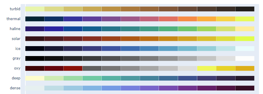
CMOcean项目的色阶
px.colors.cmocean.swatches()
Output
还有其他很多调色板供选择,就不一一展示了,下面只给出代码,具体颜色样式可以自行运行代码查看
ColorBrewer2项目的色阶
px.colors.colorbrewer
周期性色标,适用于具有自然周期结构的连续数据
px.colors.cyclical
分散色标,适用于具有自然中点的连续数据
px.colors.diverging
定性色标,适用于没有自然顺序的数据
px.colors.qualitative
顺序色标,适用于大多数连续数据
px.colors.sequential
Plotly Express 基本绘图
散点图
Plotly 绘制散点图非常容易,一行代码就可以完成
px.scatter(gap2007, x="gdpPercap", y="lifeExp")
Output
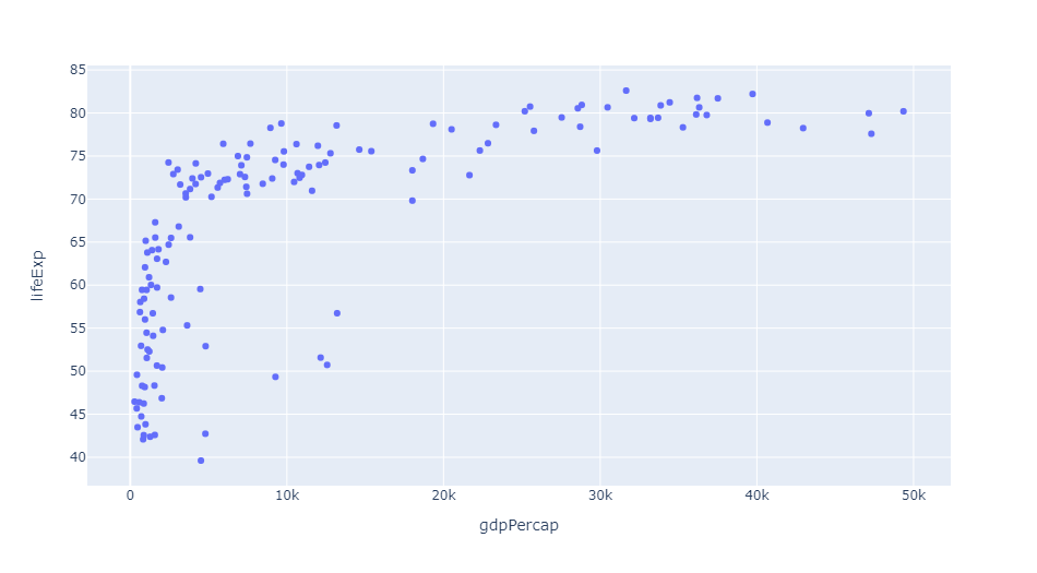
还可以通过参数 color 来区分不同的数据类别
px.scatter(gap2007, x="gdpPercap", y="lifeExp", color="continent")
Output

这里每个点都代表一个国家,不同颜色则代表不同的大洲
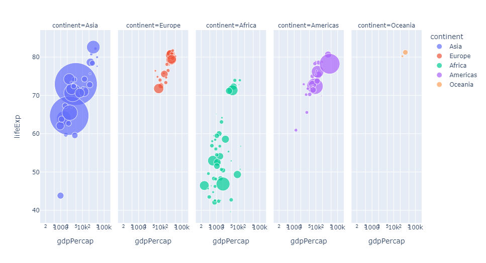
还可以使用参数 size 来体现数据的大小情况
px.scatter(gap2007, x="gdpPercap", y="lifeExp", color="continent", size="pop", size_max=60)
Output
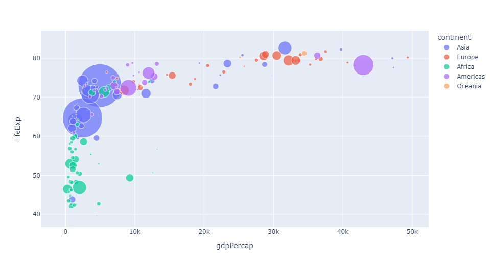
还可以通过参数 hover_name 来指定当鼠标悬浮的时候,展示的信息

还可以根据数据集中不同的数据类型进行图表的拆分
px.scatter(gap2007, x="gdpPercap", y="lifeExp", color="continent", size="pop",
           size_max=60, hover_name="country", facet_col="continent", log_x=True)
Output
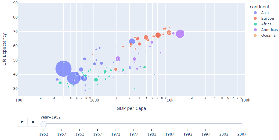
我们当然还可以查看不同年份的数据,生成自动切换的动态图表
px.scatter(gap, x="gdpPercap", y="lifeExp", color="continent", size="pop",
           size_max=60, hover_name="country", animation_frame="year", animation_group="country", log_x=True,
          range_x=[100, 100000], range_y=[25, 90], labels=dict(pop="Population", gdpPercap="GDP per Capa", lifeExp="Life Expectancy"))
Output
地理信息图
Plotly 绘制动态的地理信息图表也是非常方便,通过这种地图的形式,我们也可以清楚的看到数据集中缺少前苏联的相关数据
px.choropleth(gap, locations="iso_alpha", color="lifeExp", hover_name="country", animation_frame="year",
              color_continuous_scale=px.colors.sequential.Plasma, projection="natural earth")
Output

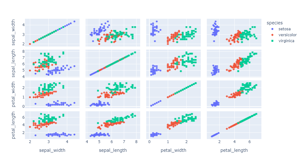
矩阵散点图
px.scatter_matrix(iris, dimensions=['sepal_width', 'sepal_length', 'petal_width', 'petal_length'], color='species', symbol='species')
Output
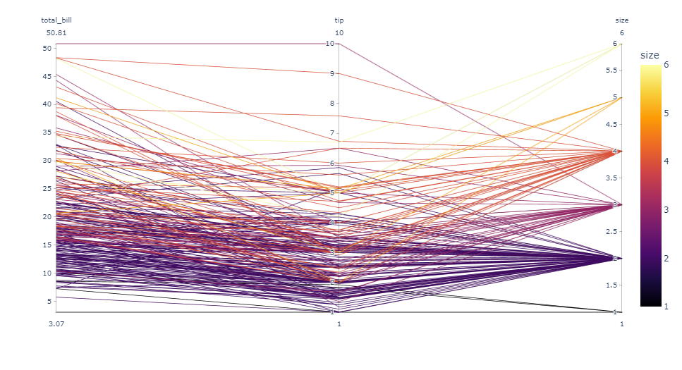
平行坐标图
px.parallel_coordinates(tips, color='size', color_continuous_scale=px.colors.sequential.Inferno)
Output
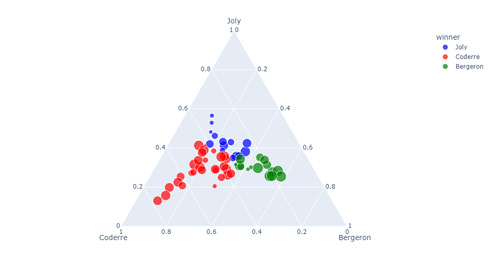
三元散点图
px.scatter_ternary(election, a="Joly", b="Coderre", c="Bergeron", color="winner", size="total", hover_name="district",
                   size_max=15, color_discrete_map = {

    "Joly": "blue",
                   "Bergeron": "green", "Coderre":"red"} )
Output
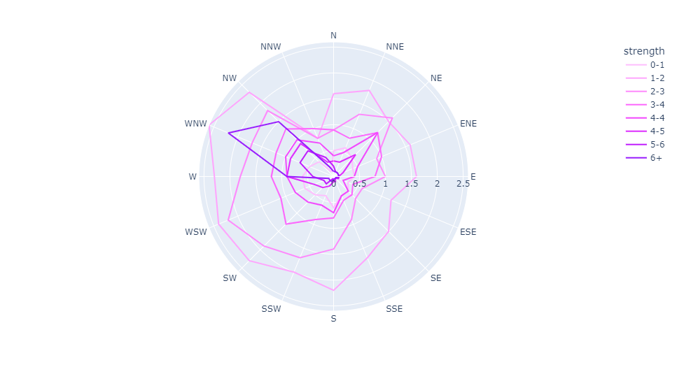
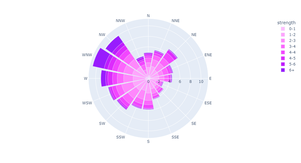
极坐标线条图
px.line_polar(wind, r="frequency", theta="direction", color="strength",
            line_close=True,color_discrete_sequence=px.colors.sequential.Plotly3[-2::-1])
Output
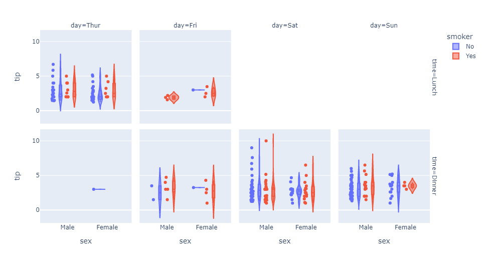
小提琴图
px.violin(tips, y="tip", x="sex", color="smoker", facet_col="day", facet_row="time",box=True, points="all",
          category_orders={

    "day": ["Thur", "Fri", "Sat", "Sun"], "time": ["Lunch", "Dinner"]},
          hover_data=tips.columns)
Output
极坐标条形图
px.bar_polar(wind, r="frequency", theta="direction", color="strength",
            color_discrete_sequence= px.colors.sequential.Plotly3[-2::-1])
Output
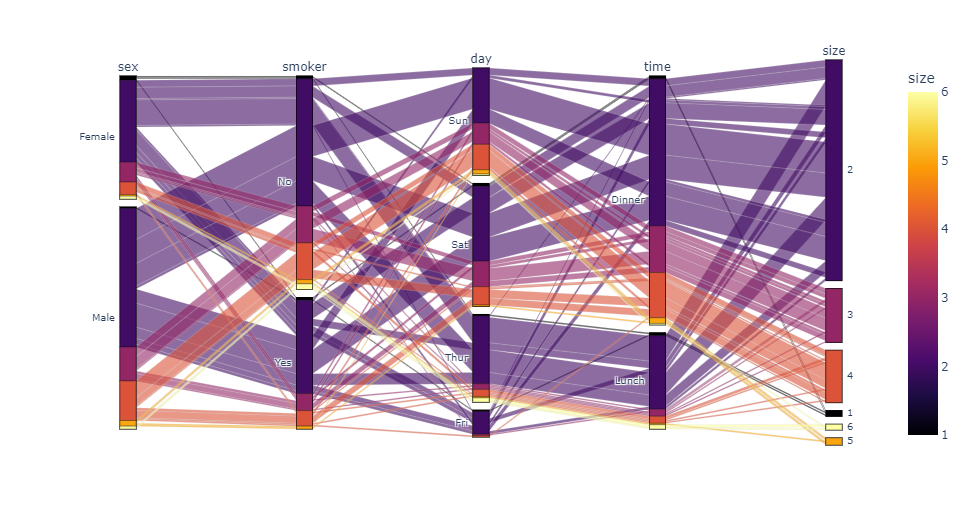
并行类别图
px.parallel_categories(tips, color="size", color_continuous_scale=px.
            colors.sequential.Inferno)
Output
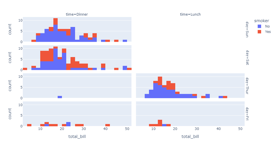
直方图
px.histogram(tips, x="total_bill", color="smoker",facet_row="day", facet_col="time")
Output
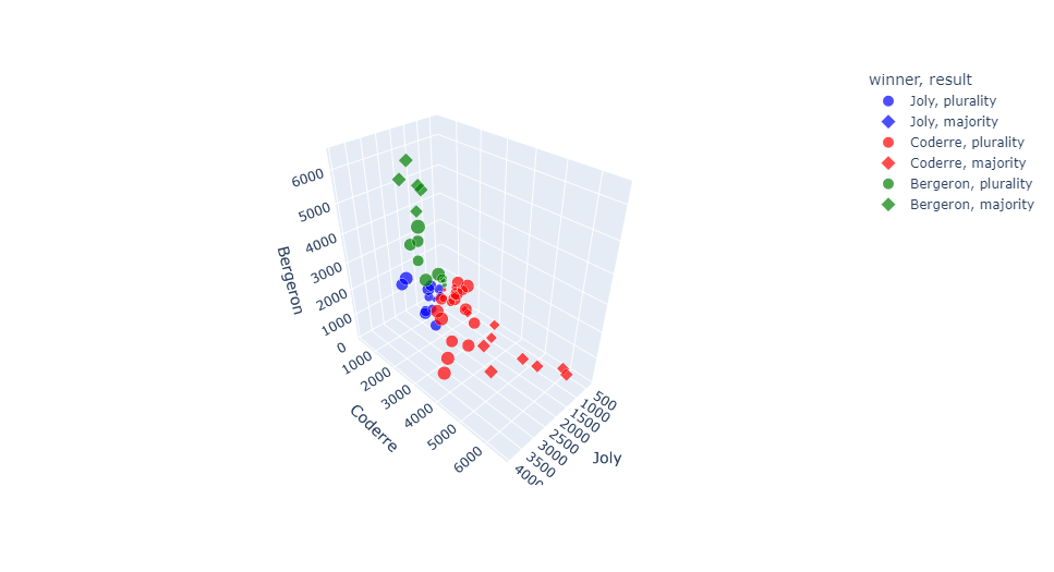
三维散点图
px.scatter_3d(election, x="Joly", y="Coderre", z="Bergeron", color="winner",
              size="total", hover_name="district",symbol="result",
              color_discrete_map = {

    "Joly": "blue", "Bergeron": "green",
              "Coderre":"red"})
Output
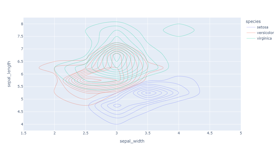
密度等值线图
px.density_contour(iris, x="sepal_width", y="sepal_length", color="species")
Output
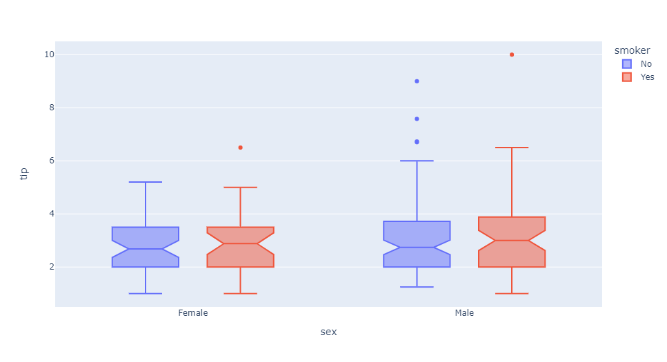
箱形图
px.box(tips, x="sex", y="tip", color="smoker", notched=True)
Output
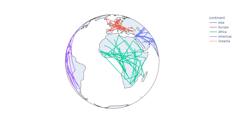
地理坐标线条图
px.line_geo(gap.query("year==2007"), locations="iso_alpha",
            color="continent", projection="orthographic")
Output
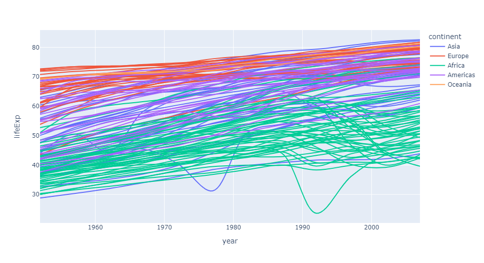
条线图
px.line(gap, x="year", y="lifeExp", color="continent",
        line_group="country", hover_name="country",
        line_shape="spline", render_mode="svg")
Output
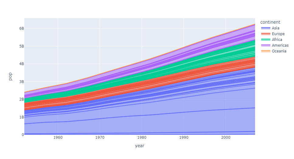
面积图
px.area(gap, x="year", y="pop", color="continent",
        line_group="country")
Output
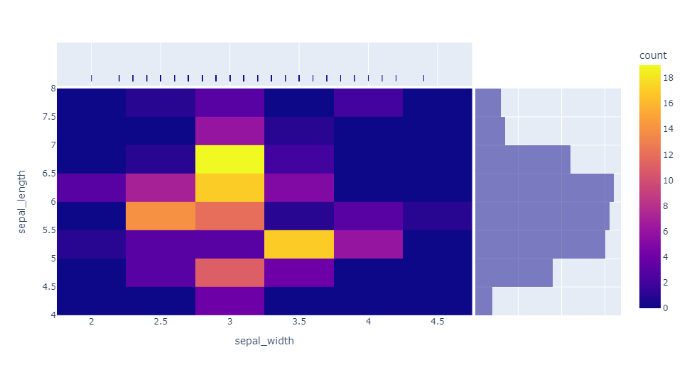
热力图
px.density_heatmap(iris, x="sepal_width", y="sepal_length",
                   marginal_x="rug", marginal_y="histogram")
Output
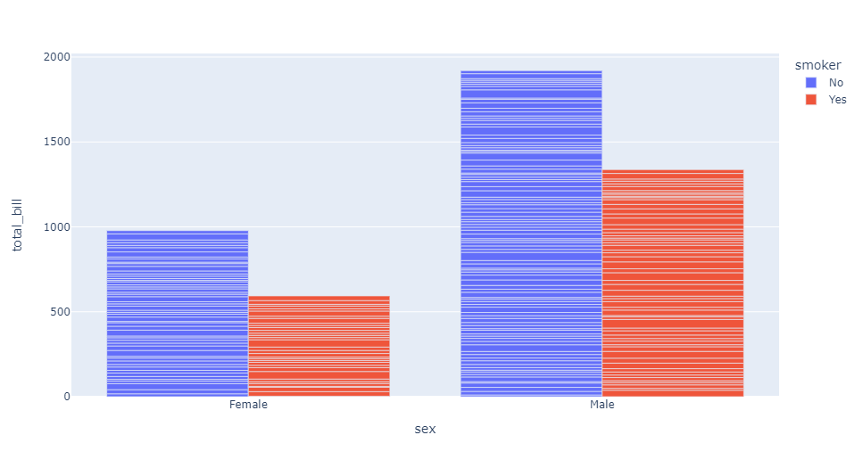
条形图
px.bar(tips, x="sex", y="total_bill", color="smoker", barmode="group")
Output
好啦,这就是今天分享的全部内容,喜欢就点个赞吧~
本文由 mdnice 多平台发布