过一遍Python的Numpy库(最后因为各种原因只过到一半)

工欲善其事，必先知其器。不了解自己使用的工具可以做哪些事，就很容易做许多费力不讨好的重复工作。

利用Python做算法，离不开科学计算，而Numpy库就是我们利用Python做科学运算时强大而基础的扩展库。

本博文对Python的Numpy库过一遍。

Numpy库提供多维数组对象、各种派生对象（如掩码数组和矩阵）以及各种用于对数组进行快速操作的例程，包括数学、逻辑、形状操作、排序、选择、I/O、离散傅立叶变换、基本线性代数、基本统计操作、随机模拟等。

NumPy 通常与 SciPy（Scientific Python）和 Matplotlib（绘图库）一起使用， 这种组合广泛用于替代 MatLab，是一个强大的科学计算环境，有助于我们通过 Python 学习数据科学或者机器学习。

• SciPy 是一个开源的 Python 算法库和数学工具包。
• SciPy 包含的模块有最优化、线性代数、积分、插值、特殊函数、快速傅里叶变换、信号处理和图像处理、常微分方程求解和其他科学与工程中常用的计算。
• Matplotlib 是 Python 编程语言及其数值数学扩展包 NumPy 的可视化操作界面。它为利用通用的图形用户界面工具包，如 Tkinter, wxPython, Qt 或 GTK+ 向应用程序嵌入式绘图提供了应用程序接口（API）。

NumPy官方链接：
NumPy官网 http://www.numpy.org/
NumPy官方文档链接 https://numpy.org/doc/stable/
NumPy 源代码：https://github.com/numpy/numpy

接下来就根据根据官方文档把Python的Numpy库过一遍。

01-官方文档主页的四个部分

01-01-Getting Started

这一部分实际上是User Guide的一部分，看下面的链接和目录就清楚了。
Getting Started的文档URL链接：
https://numpy.org/doc/stable/user/absolute_beginners.html
User Guide的文档URL链接：
https://numpy.org/doc/stable/user/index.html

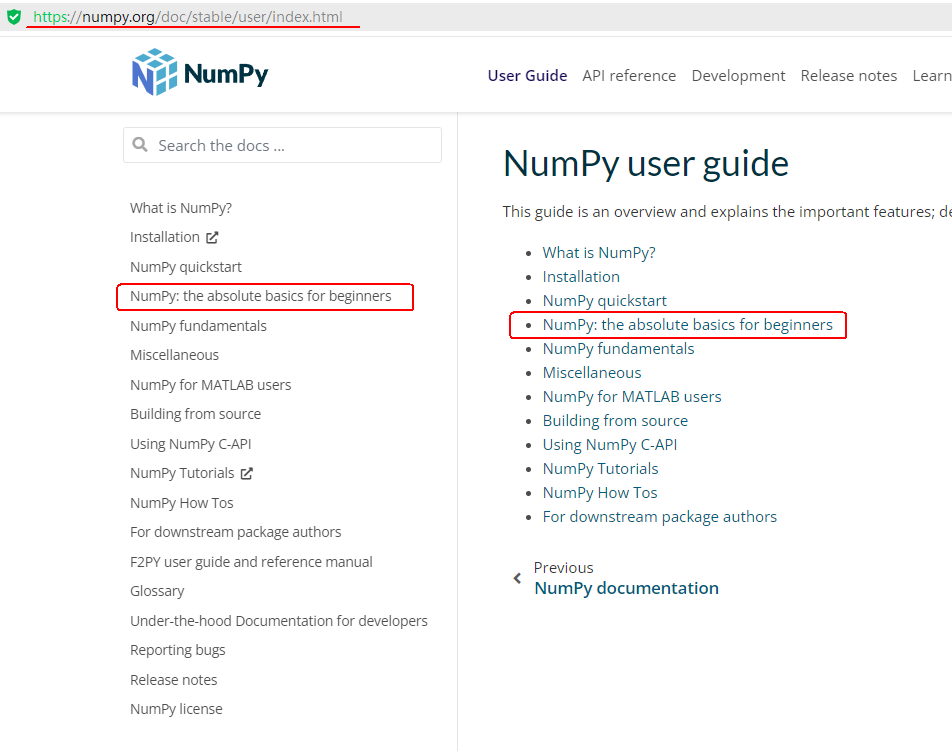
上图中红框的部分就是Getting Started的内容。
红框中的具体内容为：
NumPy: the absolute basics for beginners
也就是说它介绍的内容为Numpy库最基础的、最重要的概念和内容。
由于自己已经使用过Numpy库一段时间了，所以这部分内容可以先略过。

01-02-User Guide

官方文档URL:https://numpy.org/doc/stable/user/index.html
主要内容有以下这些：

• What is NumPy?
• Installation
• NumPy quickstart
• NumPy: the absolute basics for beginners
• NumPy fundamentals
• Miscellaneous
• NumPy for MATLAB users
• Building from source
• Using NumPy C-API
• NumPy Tutorials
• NumPy How Tos
• For downstream package authors

上面的内容很好理解，也很容易想到教程中会有这些内容，所以这一部分内容也可以不用先看。

01-03-API Reference

官方文档链接：https://numpy.org/doc/stable/reference/index.html
这个是我们需要重点关注和精读的部分。
它的内容如下：
The reference guide contains a detailed description of the functions, modules, and objects included in NumPy.The reference describes how the methods work and which parameters can be used.
可见，API Reference详细描述了 Numpy库的函数、模块、对象。所以这部分我们需要重点关注和精读。
目录如下：

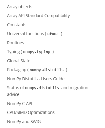
• Array objects
• Array APl Standard Compatibility
• Constants
• Universal functions ( ufunc )
• Routines
• Typing ( numpy.typing )
• Global state
• Packaging ( numpy.distutils )
• NumPy Distutils - Users Guide
• Status of numpy.distutils and migration advice
• NumPy C-API
• CPU/SIMD Optimizations
• NumPy and SWIG

01-04-Contributor’s Guide

这一部分是说如何向Numpy库作贡献，具体内容可以先略过。

接下来对API Reference的内容就行整理，结构上我会尽量保持扁平，这样遍于书写，避免结构过深，突出不了主要内容。

02-The N-dimensional array (ndarray)对象的简介、属性、方法等

02-01-ndarray对象的简介

ndarray无疑是Numpy库最重要的对象，其名字的来历为N-dimensional array。
An ndarray is a (usually fixed-size) multidimensional container of items of the same type and size.（从这句话可知ndarray对象中的元素都是相同类型和size的）

02-02-ndarray对象的属性(Attributes)

ndarray对象有以下这些属性(冒号后边表示属性的类型，请联想一个完整的类定义来理解这个问题)：
官方文档链接：https://numpy.org/doc/stable/reference/generated/numpy.ndarray.html

• T：ndarray
  The transposed array.（转置）

• data：buffer
  Python buffer object pointing to the start of the array’s data.

• dtype：dtype object
  Data-type of the array’s elements.

• flags：dict
  Information about the memory layout of the array.（这个就是指C语言还是Fortran语言的数据存储结构）

• flat：numpy.flatiter object
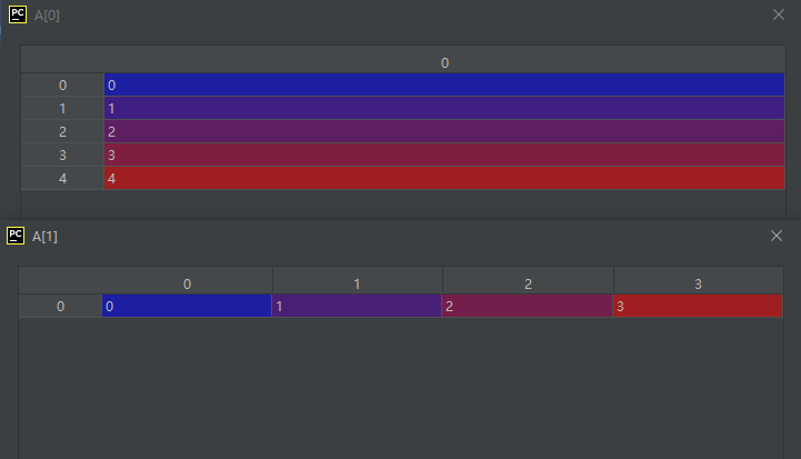
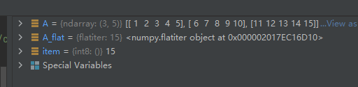
  A 1-D iterator over the array.
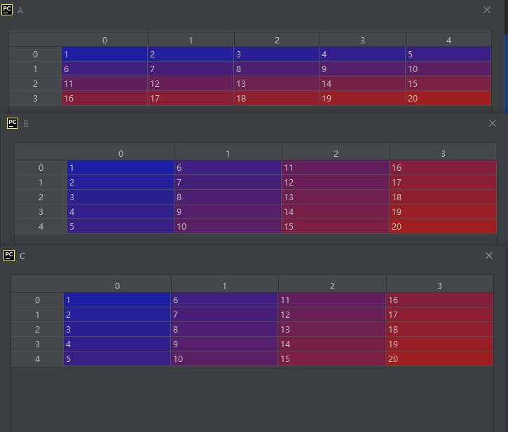
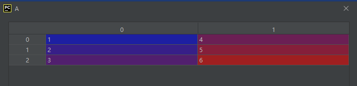
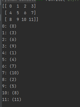
  这个是把array展平到一维空间进行迭代。什么意思？看下面这个示例：

import numpy as np

A = np.array([[1, 2, 3, 4, 5],
              [6, 7, 8, 9, 10],
              [11, 12, 13, 14, 15],
              [16, 17, 18, 19, 20]], dtype='int8')

x1 = A.flat[5]
x2 = A.flat[11]

运行结果如下：

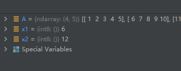
结果分析：值为6的元素按从左到右，从上到下的顺序数刚好索引为5；值为12的元素按从左到右，从上到下的顺序数刚好索引为11。
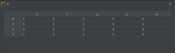
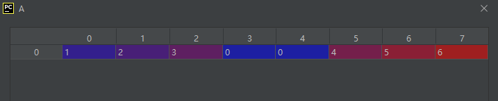
还可以利用这个属性把array的值全部置为同一个数，如下：

import numpy as np

A = np.array([[1, 2, 3, 4, 5],
              [6, 7, 8, 9, 10],
              [11, 12, 13, 14, 15],
              [16, 17, 18, 19, 20]], dtype='int8')

A.flat = 5

运行结果如下：

• ima：gndarray
  The imaginary part of the array. （复数的虚部）

• real：ndarray
  The real part of the array.（复数的实部）

• size：int
  Number of elements in the array.（元素个数总数）

• itemsize：int
  Length of one array element in bytes.（每个元素占用的内存空间大小，以字节为单位）

• nbytes：int
  Total bytes consumed by the elements of the array.（array占用的总内存空间，以字节为单位）

• ndim：int
  Number of array dimensions.

• shape：tuple of ints
  Tuple of array dimensions.(array的形状，比如三维两行四列的array的shape为(3, 2, 4))

• stride：stuple of ints
  Tuple of bytes to step in each dimension when traversing an array.

• ctypes：ctypes object
  An object to simplify the interaction of the array with the ctypes module.(用于简化阵列与ctypes模块交互的对象)

• base：ndarray
  Base object if memory is from some other object.(如果数据来自其它对象，那么这个属性表示这个其它对象的基类对象。感觉这个属性的应用并不多，关于base属性，目前并不能完全理解，比如这个base的类型为ndarray是什么鬼？？好在这个属性感觉应用的时候并不多，所以暂时也可以不求甚解)

02-02-ndarray对象的方法(Methods)

02-02-01-all():判断是否所有的元素为真

all([axis, out, keepdims, where])

Returns True if all elements evaluate to True.
判断是否所有的元素为真。

02-02-02-any():判断是否有元素为真

any([axis, out, keepdims, where])

Returns True if any of the elements of a evaluate to True.
判断是否有元素为真。

02-02-03-argmax():返回指定维度的最大索引

argmax([axis, out, keepdims])

Return indices of the maximum values along the given axis.
返回指定维度的最大索引。
示例代码如下：

import numpy as np

A = np.array([[1, 2, 3, 4, 5],
              [6, 7, 8, 9, 10],
              [11, 12, 13, 14, 15],
              [16, 17, 18, 19, 20]], dtype='int8')

max_index1 = A.argmax()
max_index2 = A.argmax(0)
max_index3 = A.argmax(1)

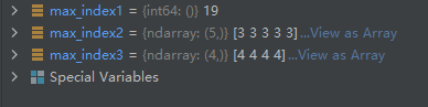
结果分析：
0代表列维度，矩阵A的每一列的索引值最大显然为3
1代表行维度，矩阵A的每一行的索引值最大显然为4
假如不指定维度，则把矩阵A按一维展平处理。

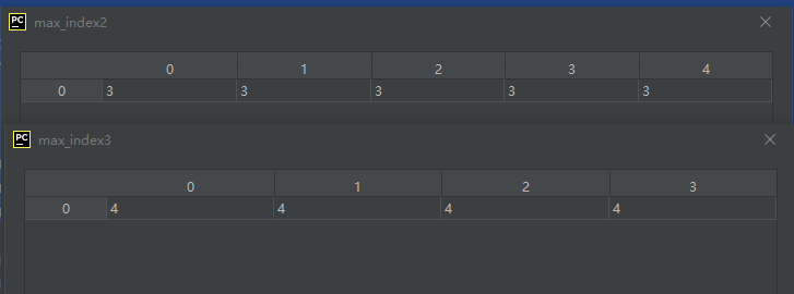
02-02-04-argmin():返回指定维度的最小索引

argmin([axis, out, keepdims])

这个昊虹君感觉有点鸡肋，通常情况下每个维度的最小索引值不应该为0么！特殊情况昊虹君是没有想到。

import numpy as np

A = np.array([[1, 2, 3, 4, 5],
              [6, 7, 8, 9, 10],
              [11, 12, 13, 14, 15],
              [16, 17, 18, 19, 20]], dtype='int8')

min_index1 = A.argmin()
min_index2 = A.argmin(0)
min_index3 = A.argmin(1)

运行结果如下：


可见，果然如昊虹君刚才分析的那样，每个维度的最小索引值都为0。

02-02-05-argpartition():partition快速排序算法【以第kth位的元素的值将数组分成两部分】

partition快速排序算法的原理是：根据一个数值x，把数组中的元素划分成两半，使得index前面的元素都不大于x，index后面的元素都不小于x。更多详情参考博文：https://blog.csdn.net/salmonwilliam/article/details/106730008
argpartition()方法的语法如下：

argpartition(kth[, axis, kind, order])

Returns the indices that would partition this array.
kth—代表数值x在数组中按从小到大的顺序处于第几位(从0开始算的第几位)

接下来举一个实际例子来说明其排序的过程：

import numpy as np

A = np.array([66, 15, 27, 33, 19, 13, 10])

partion1 = A.argpartition(3)

B = A[partion1[:]]

上面代码中方法argpartition()的排序方法如下：
首先通过某种算法找到数组A中按从小到大的顺序处于第3位的数，
数组A按从小到的顺序为：
10, 13, 15, 19, 27, 33, 66
按从小到大顺序处于第0位的数为10
按从小到大顺序处于第1位的数为13
按从小到大顺序处于第2位的数为15
按从小到大顺序处于第3位的数为19
按从小到大顺序处于第4位的数为27
按从小到大顺序处于第5位的数为33
按从小到大顺序处于第6位的数为66

所以，数组A中按从小到大的顺序处于第3位的数为19。
确定第3位数为19后，接着我们把排序后的数组的第3位置为19，然后把小于19的数扔在前面，把大于19的数扔到后面。这样形成了一个新的序列，把这个新的序列各值的原索引依次返回便得到了方法argpartition()的返回值。

上面代码的运行结果如下：

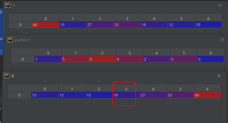
从B矩阵的内容我们可以发现，19被放在了索引值为3的位置，其前面元素的值都比19小，后面元素的值都比19大。

参数axis—表示在哪个维度上作这个排序操作，比如当axis=0时，表示对每一列进行排序操作，当axis = 1时表示对每一行进行排序操作。

import numpy as np

A = np.array([[66, 15, 27, 33, 19, 13, 10],
              [9, 8, 7, 6, 5, 4, 3]])

partion1 = A.argpartition(kth=3)

运行结果如下：

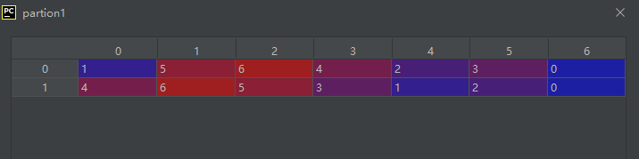
第一行中按从小到大顺序位第03位的值为19，对应索引号为4
第二行中按从小到大顺序位第03位的值为6，对应索引号为3

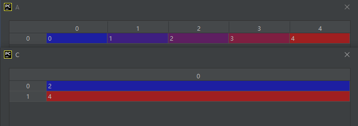
技巧：把索引值写为负数，即可得到按从大到小顺序位于第几位的元素的索引值。

另外，02-02-29有与之对应的方法partition()，partition()就是直接返回元素值了。

参考资料：
partition快速排序算法的原理：https://blog.csdn.net/salmonwilliam/article/details/106730008
实际应用示例一：https://blog.csdn.net/weixin_37722024/article/details/64440133
实际应用示例二：https://blog.csdn.net/weixin_45031468/article/details/122386360
各种排序算法总结：https://blog.csdn.net/studyeboy/article/details/113249724
Numpy库中以arg开头的排序函数：https://blog.csdn.net/studyeboy/article/details/113249724

02-02-06-argsort():对数组元素进行排序

argsort([axis, kind, order])

Returns the indices that would sort this array.

说明和示例代码略，详见博文 https://blog.csdn.net/weixin_42297347/article/details/112966004

02-02-07-astype():对array的数据类型进行转换

astype(dtype[, order, casting, subok, copy])

Copy of the array, cast to a specified type.

02-02-08-byteswap():字节交换(针对大小端问题)

byteswap([inplace])

Swap the bytes of the array elements

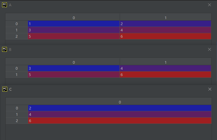
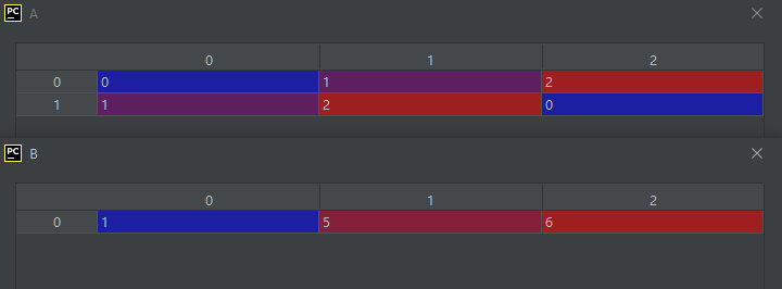
02-02-09-A.choose():以对象A中的值为索引挑选choices中的值形成新的数组

choose(choices[, out, mode])

Use an index array to construct a new array from a set of choices.
示例代码如下：

import numpy as np

A = np.array([[0, 0, 3], [1, 0, 2], [2, 1, 0]])

B = np.array([3, 7, 6, 2])

C = A.choose(B)

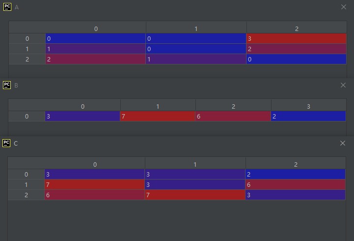
C的形成过程如下：
A[0, 0] = 0→B[0] = 3→C[0, 0] = 3
A[0, 1] = 0→B[0] = 3→C[0, 1] = 3
A[0, 2] = 3→B[3] = 2→C[0, 2] = 2

A[1, 0] = 1→B[1] = 7→C[1, 0] = 7
A[1, 1] = 0→B[0] = 3→C[1, 1] = 3
A[1, 2] = 2→B[2] = 6→C[1, 2] = 6

A[2, 0] = 2→B[2] = 6→C[2, 0] = 6
A[2, 1] = 1→B[1] = 7→C[2, 1] = 7
A[2, 2] = 0→B[0] = 3→C[2, 2] = 3

从上面的过程来看，A中各元素因为是作为对B的索引，所以A中各元素的最大值不能超过B中的最大索引数。

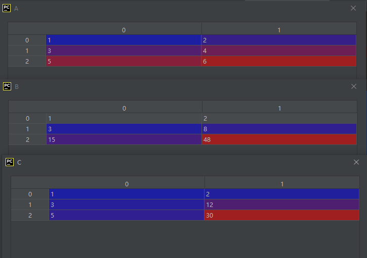
如果B是二维的，则A中各元素的值是对B中每列元素的索引：

示例如下：

A = np.array([[1, 0, 2], [0, 2, 0]])

B = np.array([[3, 7, 6],
              [1, 8, 9],
              [2, 5, 4]])

C = A.choose(B)

运行结果如下：

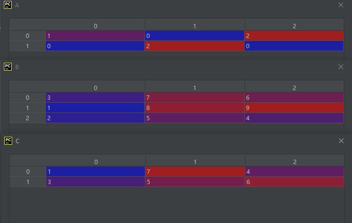
此时C的形成过程如下：
C[0,0]的值的形成过程如下：
首先我们发现A[0, 0] = 1，由于这个1位于A中的第0列，所以我们去寻找B中第0列中索引值为1的值，即B[1, 0]的值，B[1, 0] = 1，所以A[0, 0] = 1。

C[0,1]的值的形成过程如下：
首先我们发现A[0, 1] = 0，由于这个0位于A中的第1列，所以我们去寻找B中第1列中索引值为0的值，即B[0, 1]的值，B[0, 1] = 7，所以C[0, 1] = 7。

C[0,2]的值的形成过程如下：
首先我们发现A[0, 2] = 2，由于这个2位于A中的第2列，所以我们去寻找B中第2列中索引值为2的值，即B[2, 2]的值，B[2, 2] = 4，所以C[0, 2] = 4。

C[1,0]的值的形成过程如下：
首先我们发现A[1, 0] = 0，由于这个0位于A中的第0列，所以我们去寻找B中第0列中索引值为0的值，即B[0, 0]的值，B[0, 0] = 3，所以C[1, 0] = 3。

C[1,1]的值的形成过程如下：
首先我们发现A[1, 1] = 2，由于这个2位于A中的第1列，所以我们去寻找B中第1列中索引值为2的值，即B[2, 1]的值，B[2, 1] = 5，所以C[1, 1] = 5。

C[1,2]的值的形成过程如下：
首先我们发现A[1, 2] = 0，由于这个0位于A中的第2列，所以我们去寻找B中第2列中索引值为0的值，即B[0, 2]的值，B[0, 2] = 6，所以C[1, 2] = 6。

一个实际的应用场景为：
假设B为二维矩阵，每一列为一个样本，列中的元素依次为样本的某个特征值，则我们可以通过设定A取出每个样本的某个特征值形成一个新的矩阵。昊虹君窃以为02-02-43的方法take()实现这个需求更直观，更容易。

关于参数mode说两句，参数mode影响上述例子中A中各元素的取值范围，设B中的索引最大值为n-1,
则
mode=‘raise’，表示A中的数必须在[0,n-1]范围内
mode=‘wrap’，表示A中的数可以是任意的整数（signed），对n取余映射到[0,n-1]范围内
mode=‘clip’， 表示A中的数可以是任意的整数(signed)，负数映射为0，大于n-1的数映射为n-1

02-02-10-clip():把数组的值限定到[min, max]的范围

clip([min, max, out])

Return an array whose values are limited to [min, max].
原数组中小于min的值会被置为min,大于max的值被置为max，类似于饱和操作，所以这个没什么好说的。

02-02-11-compress():通过布尔值判定来对数组进行压缩处理

compress(condition[, axis, out])

示例代码如下：

import numpy as np

A = np.array([[1, 2], [3, 4], [5, 6]])

B = A.compress([0, 1, 1], axis=0)

C = A.compress([False, True], axis=1)

运行结果如下：

分析：
语句 B = A.compress([0, 1, 1], axis=0) 代表在列方向上进行压缩，第1个数0代表某列的第0个元素被舍弃；第2个数1代表某列的第1个元素被保留；第3个数1代表某列的第2个元素被保留。
以A的第0列为例，元素1被舍弃，元素3、5被保留。
以此类推…
而语句 C = A.compress([False, True], axis=1)代表在行方向上进行压缩，第1个布尔值False代表某行的第0个元素被舍弃，第2个布尔值True代表某行的第1个元素被舍弃。
以A的第0行为例，元素1被舍弃，元素2被保留。
以此类推…

02-02-12-conj():数组中各元素的共轭复数

说明和示例代码略。

02-02-13-conjugate():数组中各元素的共轭复数

同conj()

02-02-14-copy():深拷贝ndarray对象

说明和示例代码略。

02-02-15-cumprod():计算ndarray对象的累乘

cumprod([axis, dtype, out])

Return the cumulative product of the elements along the given axis.
示例代码如上：

import numpy as np

A = np.array([[1, 2], [3, 4], [5, 6]])

B = A.cumprod(axis=0)

C = A.cumprod(axis=1)

运行结果如下：

02-02-16-cumsum():计算ndarray对象的累乘

cumsum([axis, dtype, out])

Return the cumulative sum of the elements along the given axis.
这个和上一个方法很像，所以说明和示例代码略。

02-02-17-diagonal():返回由对角元素组成的数组

diagonal([offset, axis1, axis2])

注意：可通过参数offset控制返回副对角线上的元素，行列式的值的计算就要用到这个嘛。
示例代码如下：
关于函数diagonal()的详细介绍见博文：https://blog.csdn.net/wenhao_ir/article/details/125826376

02-02-18-dump():对象保存为文件

dump(file)

Dump a pickle of the array to the specified file.
单词pickle的意思为泡菜，为什么叫泡菜呢？见下面这篇博文：
https://blog.csdn.net/qq_28790663/article/details/115496733

示例代码如下：

import numpy as np

A = np.array([[1, 2],
              [3, 4]])

A.dump('./100.txt')

C = np.load('./100.txt', allow_pickle=True)

运行结果如下：


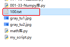
上面由dump()生成的文件100.txt的内容如下：

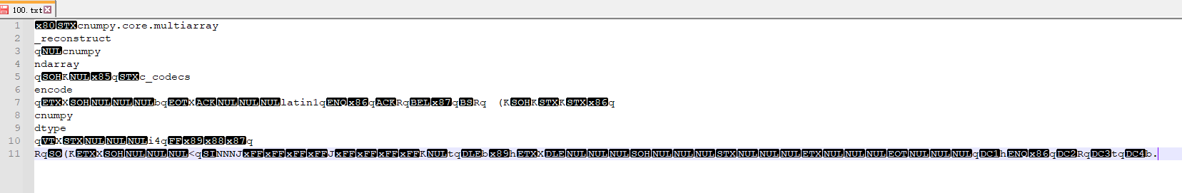
百度网盘下载链接：
https://pan.baidu.com/s/1OJ3DNcI5EIASFuDiho4HgA?pwd=8dpc

02-02-19-dumps():以字符串的形式返回pickle(泡菜)

dumps()

Returns the pickle of the array as a string.
单词pickle的意思为泡菜，为什么叫泡菜呢？见下面这篇博文：
https://blog.csdn.net/qq_28790663/article/details/115496733
实质上就是把泡菜文件的内容返回出来了，这样子的话就可以以另外的方式进行存储了。

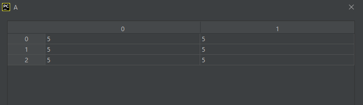
02-02-20-fill():以某个常量填充对象

fill(value)

示例代码如下：

import numpy as np

A = np.array([[1, 2],
              [3, 4],
              [5, 6]])

A.fill(5)

运行结果如下：

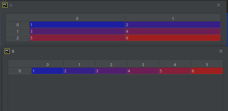
02-02-21-flatten():返回折叠(也可称为展平)为一维数组的副本

flatten([order])

order—{‘C’, ‘F’, ‘A’, ‘K’}, optional
示例代码如下：

import numpy as np

A = np.array([[1, 2],
              [3, 4],
              [5, 6]])

B = A.flatten()

运行结果如下：

02-02-22-getfield():返回对象数据中某个由数类型定义的字段的值【比如用于获取复数的实部和虚部】

getfield(dtype[, offset])

示例代码如下：

a1 = 1.+2.j
a2 = 3.+4.j
a3 = 5.+6.j
a4 = 7.+8.j

A = np.array([[a1, a2],
              [a3, a4]])

B = A.getfield(np.float64)
C = A.getfield(np.float64, offset=8)

运行结果如下：

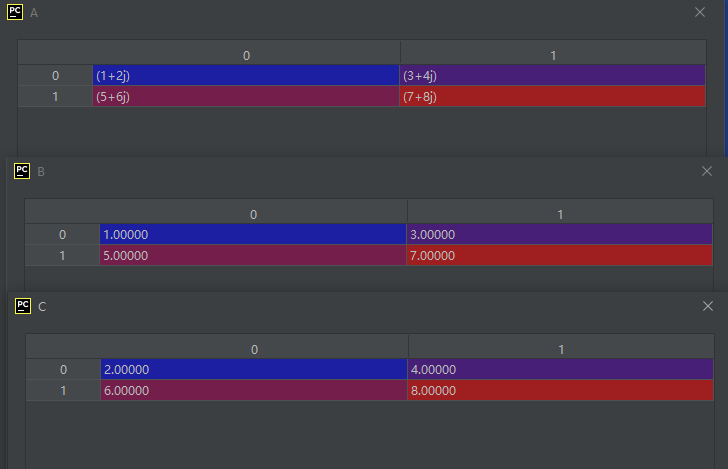
这里可以结合02-02-38-setfield()方法作进一步的认识和了解。

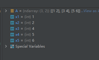
02-02-23-item():返回数组的某一个元素的值【索引一维展平化】

item(*args)

Copy an element of an array to a standard Python scalar and return it.
示例代码如下：

import numpy as np

A = np.array([[1, 2],
              [3, 4],
              [5, 6]])

x1 = A.item(0)
x2 = A.item(1)
x3 = A.item(3)
x4 = A.item(4)
x5 = A.item(5)

运行结果如下：

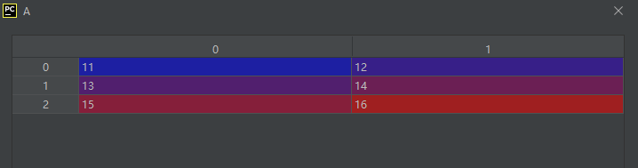
02-02-24-itemset():设置数组某一元素的值【索引一维展平化】

itemset(*args)

示例代码如下：

import numpy as np

A = np.array([[1, 2],
              [3, 4],
              [5, 6]])

A.itemset(0, 11)
A.itemset(1, 12)
A.itemset(2, 13)
A.itemset(3, 14)
A.itemset(4, 15)
A.itemset(5, 16)

运行结果如下：

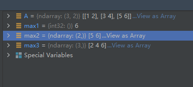
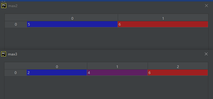
02-02-25-max():返回数组的最大值

max([axis, out, keepdims, initial, where])

Return the maximum along a given axis.
示例代码如下：

import numpy as np

A = np.array([[1, 2],
              [3, 4],
              [5, 6]])

max1 = A.max()  # 整个数组的最大值
max2 = A.max(0)  # 沿列方向求最大值,即每一列的最大值
max3 = A.max(1)  # 沿行方向求最大值,即每一行的最大值

运行结果如下：

02-02-26-mean():返回数组的平均值

mean([axis, dtype, out, keepdims, where])

Returns the average of the array elements along given axis.
因为用法同max()，所以这里就不给示例代码了。

02-02-27-min():返回数组的最小值

min([axis, out, keepdims, initial, where])

Return the minimum along a given axis.
Returns the average of the array elements along given axis.
因为用法同max()，所以这里就不给示例代码了。

02-02-28-nonzero():返回非零元素的索引

Rearranges the elements in the array in such a way that the value of the element in kth position is in the position it would be in a sorted array.

说明和示例代码：略。

02-02-29-partition():partition快速排序算法【以第kth位的元素的值将数组分成两部分】

partition(kth[, axis, kind, order])

Rearranges the elements in the array in such a way that the value of the element in kth position is in the position it would be in a sorted array.
会用argpartition()就会用这个，argpartition()的介绍见02-02-25，argpartition()返回的是索引，而这个是排好序的数组。

02-02-30-prod():计算数组内元素的乘积

prod([axis, dtype, out, keepdims, initial, ...])

Return the product of the array elements over the given axis

import numpy as np

A = np.array([[1, 2],
              [3, 4],
              [5, 6]])

prod1 = A.prod()
prod1 = A.prod(0)
prod2 = A.prod(1)

运行结果如下：


从运行结果可以看出，prod1是所有元素相乘的结果，prod2是每一列元素相乘的结果，prod3是每一行元素相乘的结果。

02-02-31-ptp():计算数组最大值与最小值之差

ptp([axis, out, keepdims])

Peak to peak (maximum - minimum) value along a given axis.
因为用法同max()，所以这里就不给示例代码了。

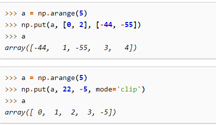
02-02-32-ptp():放置某些值到指定义的索引位置上

put(indices, values[, mode])

示例代码如下：

import numpy as np

A = np.array([[1, 2],
              [3, 4],
              [5, 6]])

A.put([0, 2], [-44, -55])

运行结果如下：

可见，索引被展平到一维空间了。

02-02-33-ravel():返回展平的一维数组

ravel([order])

Return a flattened array.

import numpy as np

A = np.array([[1, 2],
              [3, 4],
              [5, 6]])

B = A.ravel()

运行结果如下：

02-02-34-repeat():元素重复

repeat(repeats[, axis])

Repeat elements of an array.
示例代码如下：

import numpy as np

A = np.array([[1, 2],
              [3, 4],
              [5, 6]])

B = A.repeat(2, axis=0)

C = A.repeat(2, axis=1)

D = A.repeat(2)

运行结果如下：

02-02-35-reshape():把数组重塑形状

reshape(shape[, order])

Returns an array containing the same data with a new shape.
这个就不多说了，高频使用的方法。

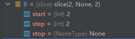
02-02-36-resize():不仅重塑形状，还可以根据新的形状增加、减少元素

resize(new_shape[, refcheck])

示例代码如下：


上面这幅截图的意思是被通过浅拷贝的数组是不允许resize()的，除非recheck的值为False。

02-02-37-round():返回每个元素按指定小数位的四舍五入值

round([decimals, out])

Return a with each element rounded to the given number of decimals.
说明和示例代码：略。

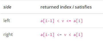
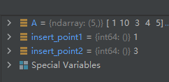
02-02-38-searchsorted():寻找某值合适的插入位置，使其比左边的值大，比右边值的小

searchsorted(v[, side, sorter])

Find indices where elements of v should be inserted in a to maintain order.
插入时满足的条件如下：

示例代码如下：

A = np.array([1, 10, 3, 4, 5])

insert_point1 = A.searchsorted(2)
insert_point2 = A.searchsorted(3, side='right')

运行结果如下：

一个应用示例是一个排好序的数组，现在要插入一个数使其不必变由小到大的顺序，那么插入到什么位置呢？就可以用方法searchsorted()确定。

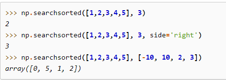
结果分析：
在第一行代码中，3插入后放到索引为2的位置不会改变原数组从小到大的顺序。
在第二行代码中，3插入后放到索引为3的位置不会改变原数组从小到大的顺序，第一行代码和第二行代码的不同在于第二行代码是从左到右寻找，而第二行代码是从右往左寻找。

02-02-38-setfield():在由类型定义的字段上放置某个值

setfield(val, dtype[, offset])

Put a value into a specified place in a field defined by a data-type.
示例代码如下：

import numpy as np

A = np.eye(3)

B = A.getfield(np.float64)

A.setfield(3, np.int32)

C = A.getfield(np.int32)
D = A.getfield(np.float64)

运行结果：

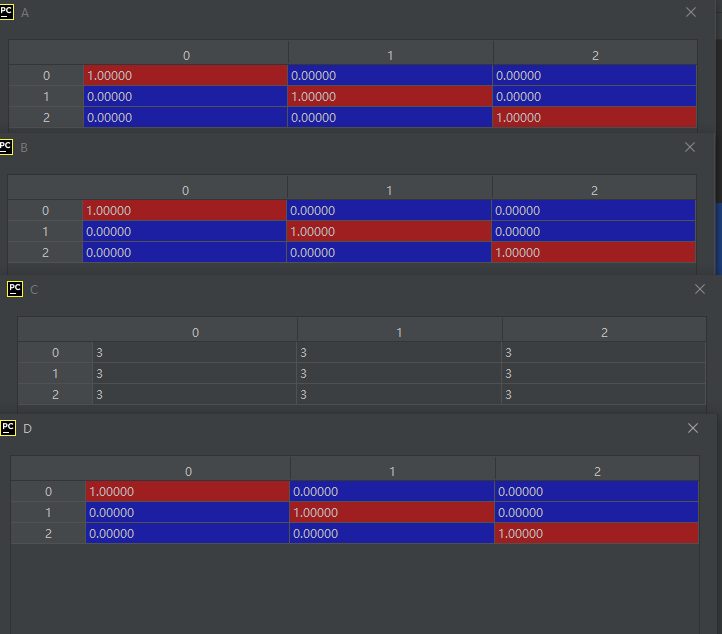
运行结果分析：
从这个运行结果我们可以看出，A中的np.int32字段值被置为3后，A仍然是一个单位矩阵，只有当我们用方法getfield()访问np.int32字段时才能得到各元素的值为3的状态。

02-02-39-setflags():设置write、align、uic的状态

setflags([write, align, uic])

这个不常用，所以略过。

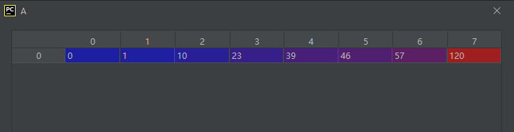
02-02-40-sort():对数组进行排序操作

sort([axis, kind, order])

示例代码如下：

import numpy as np

A = np.array([46, 57, 23, 39, 1, 10, 0, 120])

A.sort()

运行结果如下：

02-02-41-squeeze():将维度数量为1的维度去掉,从而达到简化维度的目的

squeeze([axis])

Remove axes of length one from a.

import numpy as np

A = np.arange(10).reshape(1, 10)
B = np.squeeze(A)

运行结果如下：

结果分析：A中由于只有1行，所以A中的行维度被去掉了。

再来个例子：

import numpy as np

A = np.array([1, 2, 3, 4], ndmin=3)

B = np.squeeze(A)

运行结果如下：

运行结果分析：
在创建数组A的时候，指定了它为三维的，但是第一维度和第二维度的数量都为2，所以通过squeeze()的操作，把这两个维度去掉，从而成了一维的数组。

02-02-41-std():返回标准差

std([axis, dtype, out, ddof, keepdims, where])

Returns the standard deviation of the array elements along given axis.
说明和示例代码：略。

02-02-41-sum():返回数组和

sum([axis, dtype, out, keepdims, initial, where])

Return the sum of the array elements over the given axis.

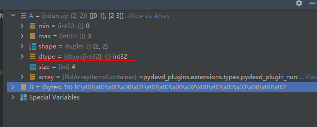
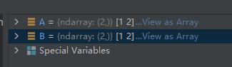
02-02-42-swapaxes(axis1, axis2):返回维度交换后的数组视图【对于二维矩阵来说，交换两个维度就相当于矩阵转置】【注意是视图，即浅拷贝(引用)】

swapaxes(axis1, axis2)

Return a view of the array with axis1 and axis2 interchanged.
示例代码如下：

import numpy as np

A = np.array([[1, 2, 3, 4, 5],
              [6, 7, 8, 9, 10],
              [11, 12, 13, 14, 15],
              [16, 17, 18, 19, 20]], dtype='int8')

B = A.swapaxes(0, 1)
C = A.swapaxes(1, 0)

运行结果如下：

在使用它时可考虑方法transpose()，两个的功能是很相似的。

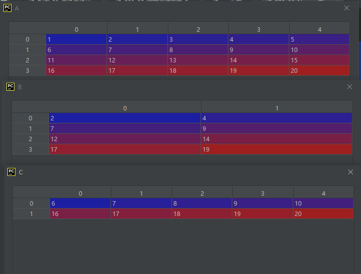
02-02-43-take():返回由指定维度指定索引的元素生成的数组

take(indices[, axis, out, mode])

Return an array formed from the elements of a at the given indices.
示例代码如下：

import numpy as np

A = np.array([[1, 2, 3, 4, 5],
              [6, 7, 8, 9, 10],
              [11, 12, 13, 14, 15],
              [16, 17, 18, 19, 20]], dtype='int8')

B = A.take([1, 3], 1)
C = A.take([1, 3], 0)

运行结果如下：

02-02-43-tobytes():把数字转化为字节表示

tobytes([order])

Construct Python bytes containing the raw data bytes in the array.

示例代码如下:

import numpy as np

A = np.array([[0, 1], [2, 3]])

B = A.tobytes()

运行结果如下：

A中的每个元素占32/8=4个字节，A中有四个元素，所以B由16个字节数组成。

02-02-44-tofile():将数组转化为文件

tofile(fid[, sep, format])

Write array to a file as text or binary (default).

说明和示例代码：略。

02-02-45-tofile():将数组转化为列表(list)

tolist()

02-02-45-tostring():把数字转化为字节表示【同tobytes()】

tostring([order])

A compatibility alias for tobytes, with exactly the same behavior.
说明和示例代码：略。

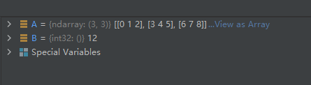
02-02-45-trace():返回对角线上元素的和

trace([offset, axis1, axis2, dtype, out])

Return the sum along diagonals of the array.

示例代码如下：

import numpy as np

A = np.array([[0, 1, 2],
              [3, 4, 5],
              [6, 7, 8]])

sum_1 = A.trace()

运行结果如下：

02-02-45-transpose():返回数组的转置视图【通过改变维度轴axis来实现】【注意是视图，即浅拷贝】

transpose(*axes)

Returns a view of the array with axes transposed.
示例代码如下：

import numpy as np

A = np.array([[0, 1, 2],
              [3, 4, 5]])

B = A.transpose()

C = A.transpose((1, 0))

D = A.transpose((0, 1))

运行结果如下：

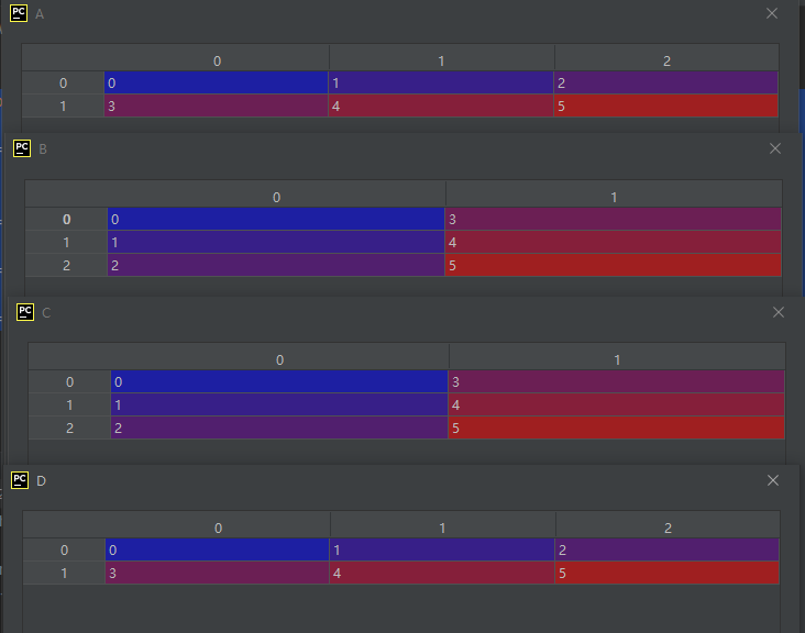
怎么理解上面的结果呢？
先说C是怎么生成的。

C = A.transpose((1, 0))

首先要知道1代表行维度，0代表列维度。
本来一个点在直角坐标系中的坐标值顺序应该是横坐标在前(列维度的索引，比如第3列的点其横坐标为3)，纵坐标在后(行维度的索引，比如第4行的点其纵坐标为4)，写成元组其顺序为(0, 1)，但是现在生成C的元组参数为(1, 0)，相当于把行和列进行了一次交换，从而得到了转置。

当transpose()不写参数时，默认把正常的维度顺序进行反转，比如正常的维度顺序为(0, 1)那么反转后为(1,0)，正常的维度顺序为(0, 1 ,2)那么反转后为(2, 1, 0)。 这样就有了B和C的结果一样。

到于D，正常的维度坐标顺序为(0, 1)，它的参数也是(0, 1)，所以相当于是不做任何操作。

注意是浅拷贝，示例如下：

import numpy as np

A = np.array([[0, 1, 2],
              [3, 4, 5]])

B = A.transpose()

C = A.transpose((1, 0))

D = A.transpose((0, 1))

D[0, 1] = 88

运行结果如下：

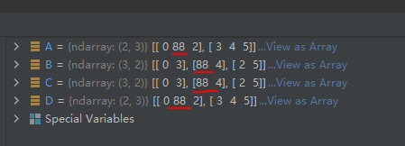
在使用它时可考虑方法swapaxes()，两个的功能是很相似的。

02-02-45-var():计算数组的方差

var([axis, dtype, out, ddof, keepdims, where])

Returns the variance of the array elements, along given axis.

02-02-46-view():返回数组的一个视图(view)【浅拷贝】

view([dtype][, type])

New view of array with the same data.
说明和示例代码略。

03-Numpy中的标量对象(Scalars)

这部分的官方文档：https://numpy.org/doc/stable/reference/arrays.scalars.html
这部分内容刚才大致浏览了下，就目前的状态，没必要去做细致了解。
知道以下几点就可：

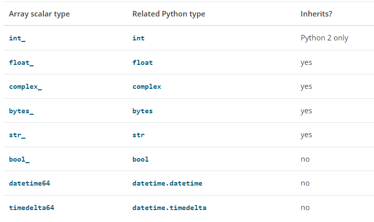
• Numpy中的数据类型，比如uni8、int32、float32等都是标量类，每一个具体的标量都是这些标量类的实例化对象，Numpy中的数据类型有一部分继承于Python的内建标量类(如下图所示)。对于Python而言，其每一个标量也可看成是一个对象，比如 x1 =3.0 则x1是浮点类float的一个实例化对象，这个对象的值属性为3.0。
  
• Numpy中的各标量类的继承关系如下：
  
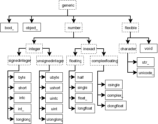
  从上图的关系图可以看出，类generic为所有标量类的基类，类number为所有数值类的基类。所以如果想细致学习这部分内容，那么我们首先应该把类generic和类number的属性(Attributes)和方法(Methods)搞清楚，再去了解具体某个标量类的属性(Attributes)和方法(Methods)比较好。

04-数据类型对象(Data type objects)

这类对象用于表示和管理Numpy中的数据类型，综合考虑，这部分内容暂时不用深入了解。

05-与索引有关的操作方法(Indexing routines)

05-01-Generating index arrays(生成数组索引的操作)

05-01-01-c_:将切片对象转换为沿第二个轴(axis)连接

示例代码如下：

import numpy as np

A = np.c_[np.array([1, 2, 3]), np.array([4, 5, 6])]

结果如下：

05-01-02-r_:将切片对象转换为沿第一个轴连接

示例代码如下：

import numpy as np

A = np.r_[np.array([1, 2, 3]), 0, 0, np.array([4, 5, 6])]

运行结果如下：

05-01-02-s_:生成切片索引对象的方法

A nicer way to build up index tuples for arrays.
示例代码如下：

import numpy as np

B = np.s_[2::2]

A = np.array([0, 1, 2, 3, 4])

C = A[B]

运行结果如下：


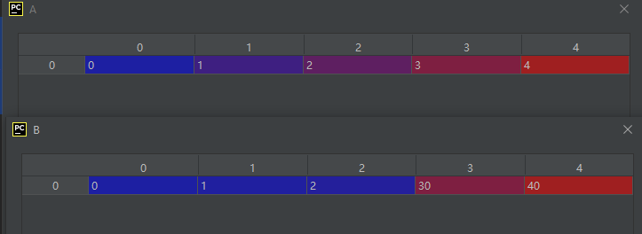
看了上面这个B对象的结构大家就应该知道语句np.s_[2::2]的作用了，实际上就是三冒号规则，详情见：https://blog.csdn.net/wenhao_ir/article/details/123034635

05-01-03-nonzero(a):返回对象a的非零(非0)元素索引

说明和示例代码：略。

05-01-04-where():条件选择数组内的元素

where(condition, [x, y], /)

用where实现饱和操作的示例代码见博文：
https://blog.csdn.net/wenhao_ir/article/details/125296528

再附一个示例代码如下：

import numpy as np

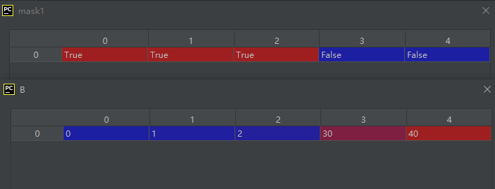
A = np.array([0, 1, 2, 3, 4])

B = np.where(A < 3, A, 10*A)

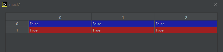
补充说明：A < 3实际上是一个掩码数组(掩码矩阵)，第二个参数为掩码值为True时A中对应元素的操作，第三个参数为掩码值为False时A中对应元素的操作，显然整个过程对A中元素执行了迭代操作。所以代码也可写成下面这样：

import numpy as np

A = np.array([0, 1, 2, 3, 4])

mask1 = A < 3

B = np.where(mask1, A, 10*A)

运行结果如下：

在实际使用时可以考虑的相似函数见博文 https://blog.csdn.net/wenhao_ir/article/details/125834005

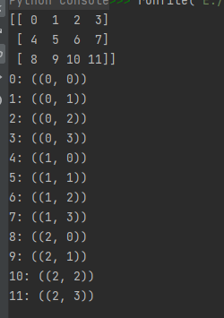
05-01-05-indices():返回某个形状(shape)矩阵的索引矩阵

indices(dimensions[, dtype, sparse])

Return an array representing the indices of a grid.

示例代码如下：

import numpy as np

index_array = np.indices((2, 3))

运行结果如下：



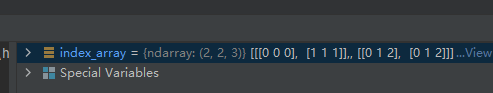
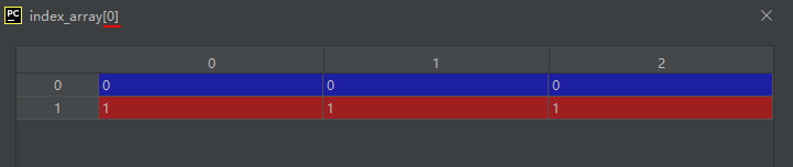
结果分析：
(2, 3)代表一个二维的矩阵，设这个矩阵为A，则A矩阵有两行三列。
则其每个元素的索引由两个数构成，所以inde_array由两个两行三列的矩阵构成。
具体来说：

A[0,0]的索引号为(inde_array[0][0,0], inde_array[1][0,0])
A[0,1]的索引号为(inde_array[0][0,1], inde_array[1][0,1])
A[0,2]的索引号为(inde_array[0][0,2], inde_array[1][0,2])
A[1,0]的索引号为(inde_array[0][1,0], inde_array[1][1,0])
A[1,1]的索引号为(inde_array[0][1,1], inde_array[1][1,1])
A[1,2]的索引号为(inde_array[0][1,2], inde_array[1][1,2])

05-01-06-ix_(*args):建立网格(mesh)索引

ix_(*args)

Construct an open mesh from multiple sequences.
示例代码如下：

import numpy as np

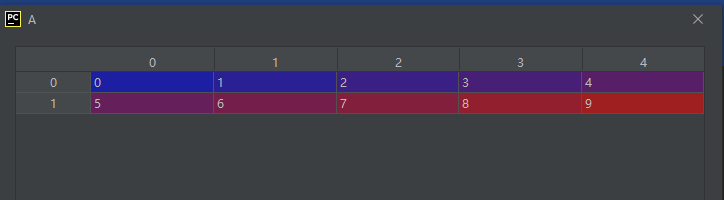
A = np.arange(10).reshape(2, 5)

ixgrid = np.ix_([0, 1], [2, 4])

B = A[ixgrid]

运行结果如下：


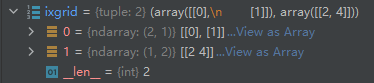
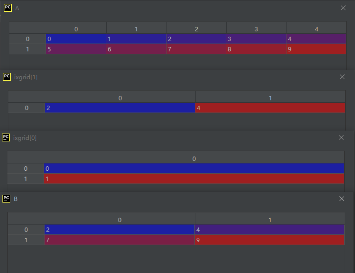
结果分析：
由上面的结果我们可以看出，由np.ix_()生成的索引遵循以下规律，第一个列表型参数转化为一个列向量，代表被选中的元素的行号；第二个列表型参数不变，仍然是一个行向量，代表被选中的元素的行号。为什么是一个行向量，一个列向量，可以从其说明中来理解：“Construct an open mesh from multiple sequences.”注意关键词“mesh”，“mesh”为网格的意思，纵横交错才能形成网格嘛。
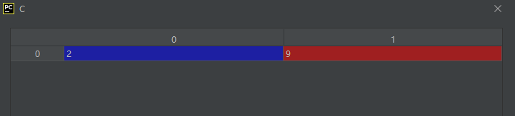
和下面这种索引方法对比一下，会更容易记忆、理解和区分：

import numpy as np

A = np.arange(10).reshape(2, 5)

C = A[[0, 1], [2, 4]]

运行结果如下：


参考资料：https://blog.csdn.net/qq_30230591/article/details/105387361

05-01-07-ogrid():生成多维数组的网格

ogrid

nd_grid instance which returns an open multi-dimensional “meshgrid”.
示例代码如下：

import numpy as np

A = np.ogrid[0:5, 0:4]

运行结果如下：

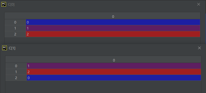
05-01-08-ravel_multi_index():返回指定元素的一维展平(flat)索引

ravel_multi_index(multi_index, dims[, mode, ...])

Converts a tuple of index arrays into an array of flat indices, applying boundary modes to the multi-index.
示例代码如下：

import numpy as np

A = np.array([[0, 1, 2], [1, 2, 0]])
B = np.ravel_multi_index(A, (3, 3))

运行结果如下：

结果分析：
由A中的两个list可组成以下三个元素的索引，(0, 1)、(1, 2)、(2, 0)
这三个点在元组(3, 3)代表的3行3列数组中，按从左到右，从上到下的顺序数，刚好位置索引是1、5、6。

05-01-09-ravel_multi_index():这个刚好和上一个函数互为反函数(将展平的索引变为多维的索引)

ravel_multi_index(multi_index, dims[, mode, ...])

Converts a tuple of index arrays into an array of flat indices, applying boundary modes to the multi-index.
示例代码如下：

import numpy as np

A = np.array([[0, 1, 2], [1, 2, 0]])
B = np.ravel_multi_index(A, (3, 3))

C = np.unravel_index(B, (3, 3))

运行结果如下：

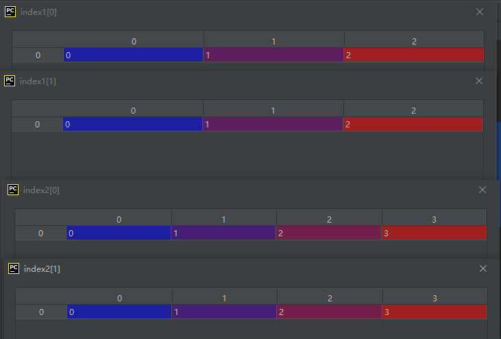
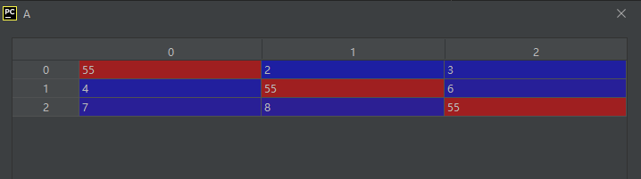
05-01-10-diag_indices():返回指定维度数的矩阵的主对角线的索引

diag_indices(n[, ndim])

Return the indices to access the main diagonal of an array.
说明和示例代码见下面这个函数。

05-01-11-diag_indices_from():返回指定矩阵的主对角线的索引

diag_indices_from(arr)

Return the indices to access the main diagonal of an n-dimensional array.
diag_indices()和diag_indices_from()都是返回主对角线的索引，那么二者有什么区别呢？主要是二者输入参数的不同，前者是多维矩阵每一维的阶数，后者是具体的矩阵。
示例代码如下：

import numpy as np

index1 = np.diag_indices(3)
index2 = np.diag_indices(4)

A = np.array([[1, 2, 3], [4, 5, 6], [7, 8, 9]])

index3 = np.diag_indices_from(A)

A[index3] = 55

运行结果如下：

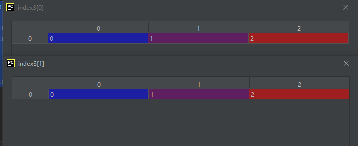
05-01-12-mask_indices():通过调用mask_fun生成mask(掩码矩阵)索引

mask_indices(n, mask_func[, k])

Return the indices to access (n, n) arrays, given a masking function.
示例代码如下：

import numpy as np

iu = np.mask_indices(3, np.triu)

运行结果如下：

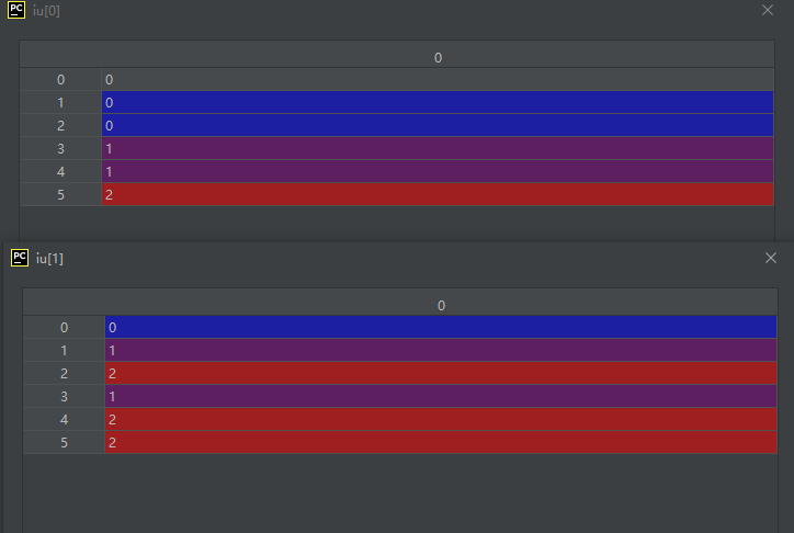
结果分析：参数np.triu代表返回矩阵的上三角矩阵，所以语句

iu = np.mask_indices(3, np.triu)

会返回三阶mask的上三角元素的索引。
由返回的iu的两个元素，我们可以得到以下六个元素的坐标
(0, 0)
(0, 1)
(0, 2)
(1, 1)
(1, 2)
(2, 2)
把这六个点在三阶矩阵中标出来，位置如下：

可见，刚好是矩阵的上三角矩阵。
补充说明一下：mask_func—是类似于triu, tril之类的函数，triu返回上三角矩阵， tril返回下三角矩阵，主要特点是部分元素的bool值为false，而另一部分元素的bools值为true。

05-01-13-tril_indices(n[, k, m]):返回形状为(n,m)的下三角矩阵索引

tril_indices(n[, k, m])

Return the indices for the lower-triangle of an (n, m) array.
说明和示例代码略。

05-01-14-tril_indices_from(arr[, k]):返回数组arr的下三角矩阵索引

tril_indices_from(arr[, k])

Return the indices for the lower-triangle of arr.

05-01-15-triu_indices(n[, k, m])：返回形状为(n,m)的上三角矩阵索引

triu_indices(n[, k, m])

Return the indices for the upper-triangle of an (n, m) array.

05-01-16-triu_indices_from(arr[, k])：返回数组arr的上三角矩阵索引

triu_indices_from(arr[, k])

Return the indices for the upper-triangle of arr.

05-02-Indexing-like operations(通过索引由一个矩阵生成另一个矩阵的操作)

05-02-01-take():由索引从一个矩阵挑选元素得到另一个矩阵

take(a, indices[, axis, out, mode])

Take elements from an array along an axis.
这个函数之前在02-02-43-take()已经详细介绍过了,示例也到02-02-43-take()中去看吧！

05-02-02-take_along_axis():由索引从一个矩阵挑选元素得到另一个矩阵(索引可以是二维以上数组)

函数take_along_axis()很不好理解，为些，我专门写了篇博文，链接：https://blog.csdn.net/wenhao_ir/article/details/125819211

05-02-03-choose(a, choices[, out, mode]):前面已介绍过

choose(a, choices[, out, mode])

Construct an array from an index array and a list of arrays to choose from.

这个函数在02-02-09-A.choose()中已经介绍过了。

05-02-04-compres():前面已介绍过

compress(condition, a[, axis, out])

Return selected slices of an array along given axis.
这个函数在02-02-11-compress()中已经介绍过了。

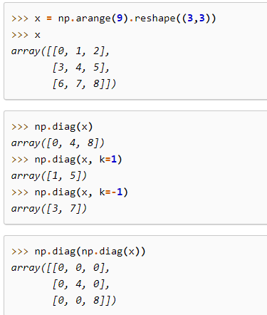
05-02-05-diag(v[, k]):返回对角线上元素的值(主对角线、副对角线都可以)

diag(v[, k])

Extract a diagonal or construct a diagonal array.
官方给的示例代码如下：

05-02-06-diagonal(a[, offset, axis1, axis2]):返回对角线元组(可处理多维数组,比如三维以上数组)

关于函数diagonal()的详细介绍见博文：https://blog.csdn.net/wenhao_ir/article/details/125826376

05-02-07-select(condlist, choicelist[, default]):根据条件对元素作相应操作

select(condlist, choicelist[, default])

Return an array drawn from elements in choicelist, depending on conditions.

示例代码如下：

x = np.arange(6)
condlist = [x<3, x>3]
choicelist = [x, x**2]
np.select(condlist, choicelist, 42)
array([ 0,  1,  2, 42, 16, 25])

要注意第三个参数的意义：
defaultscalar, optional
The element inserted in output when all conditions evaluate to False.
在实际使用时可以考虑的相似函数或方法见博文：https://blog.csdn.net/wenhao_ir/article/details/125834005

05-02-28-lib.stride_tricks.sliding_window_view(x, …):创建数组的滑动窗口索引数组视图(view)

lib.stride_tricks.sliding_window_view(x, ...)

Create a sliding window view into the array with the given window shape.

这个函数是做图像处理工作同学的福音啊，图像处理算法里面有大量的窗运算这是众所周知的。

示例代码如下：

# -*- coding: utf-8 -*-

import numpy as np
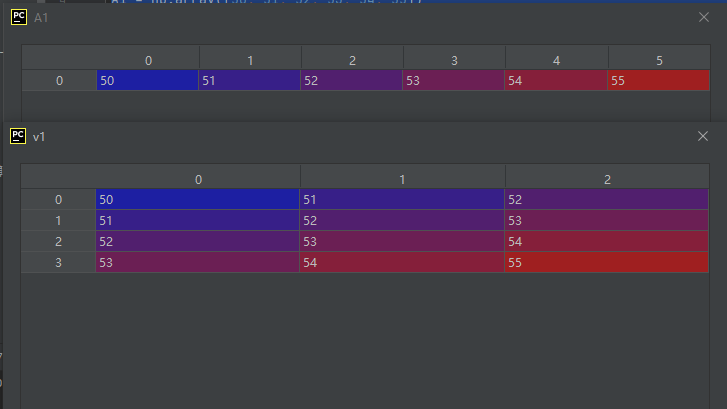
A1 = np.array([50, 51, 52, 53, 54, 55])

v1 = np.lib.stride_tricks.sliding_window_view(A1, 3)

运行结果如下：

要注意：既然是view，那么就是浅拷贝哦！

再来个二维数组的实例：

# -*- coding: utf-8 -*-

import numpy as np
A1 = np.array([[50, 51, 52, 53],
              [54, 55, 56, 57]])

v1 = np.lib.stride_tricks.sliding_window_view(A1, (2, 2))

运行结果如下：


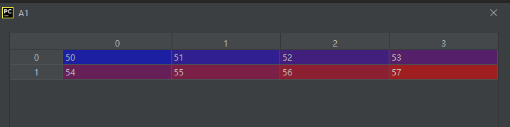
是不是帅呆了…有了这个函数以后实现与窗口算法有关的操作就方便多啦~

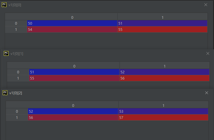
05-02-29-lib.stride_tricks.as_strided(x[, shape, …]):创建矩阵的跨步视图(view)【类似于通过控制shape和stride得到子矩阵】

lib.stride_tricks.as_strided(x[, shape, ...])

Create a view into the array with the given shape and strides.

import numpy as np
A1 = np.array([[50, 51, 52, 53],
              [54, 55, 56, 57]])

v1 = np.lib.stride_tricks.as_strided(A1, shape=(2, 2), strides=None, subok=False, writeable=True)

运行结果如下：

05-03-通过索引向数组插入数据(Inserting data into arrays)

05-03-01-place(arr, mask, vals):通过掩码数组的真假值插入数据

place(arr, mask, vals)

Change elements of an array based on conditional and input values.
示例代码如下：

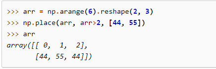
要注意arr>2实际上是一个数组，如下：

import numpy as np

arr = np.arange(6).reshape(2, 3)

mask1 = arr > 2

运行结果如下：

05-03-02-put(a, ind, v[, mode]):放置指定值到由索引指定的位置【索引是一维展平(flat)索引】

put(a, ind, v[, mode])

Replaces specified elements of an array with given values.

05-03-03-put_along_axis():沿指定维度(axis)放置指定值到指定位置

put_along_axis(arr, indices, values, axis)

Put values into the destination array by matching 1d index and data slices.
注意：indices要与arr的维度数一样。

示例代码如下：

import numpy as np

A = np.array([[10, 30, 20], [60, 40, 50]])
A_max_index = np.argmax(A, axis=1)

A_max_index_expand = A_max_index[:, None]

np.put_along_axis(A, A_max_index_expand, 99, axis=1)

运行结果如下：


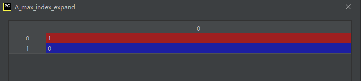
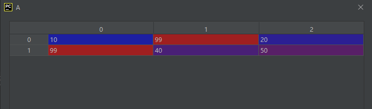
从运行结果中我们可以看出，通过上面代码的操作，把每一行中的最大值都置为了99。为了使A_max_index的维度数与A的维度数一样，进行了扩维操作。

05-03-04-putmask():通过掩码使得掩码值为True的元素的值按一定的操作改变

putmask(a, mask, values)

Changes elements of an array based on conditional and input values.
示例代码如下：

import numpy as np

x = np.arange(6).reshape(2, 3)
mask1 = x > 2
np.putmask(x, mask1, x**2)

运行结果如下：

注意：上面的语句

np.putmask(x, mask1, x**2)

也可以写为：

np.putmask(x, x > 2, x**2)

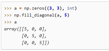
05-03-05-fill_diagonal(a, val[, wrap]) 以某个值填充对角线元素

fill_diagonal(a, val[, wrap])

Fill the main diagonal of the given array of any dimensionality.
示例代码如下：

05-04-Iterating over arrays(与索引有关的数组迭代操作)

05-04-01-nditer():迭代ndarray对象中的每一个元素

nditer(op[, flags, op_flags, op_dtypes, ...])

Efficient multi-dimensional iterator object to iterate over arrays.
示例代码如下：

import numpy as np

a = np.arange(6).reshape(2, 3)
for x in np.nditer(a):
    print(x)

运行结果如下：

关于上面这个示例代码中的for循环及内置函数中类似的操作，可参考博文 https://blog.csdn.net/wenhao_ir/article/details/125443427

关于函数nditer()的详细说明可参考博文：https://blog.csdn.net/jiangjiang_jian/article/details/77540599

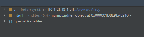
实际上函数nditer()返回了一个nditer迭代对象，nditer对象也是Numpy库的一个对象类型。

import numpy as np

a = np.arange(6).reshape(2, 3)
inter1 = np.nditer(a)

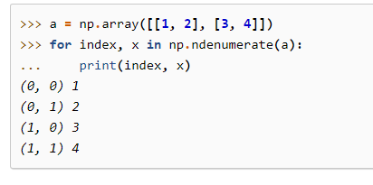
05-04-02-ndenumerate(arr):枚举化迭代

ndenumerate(arr)

Multidimensional index iterator.
这个就根我在博文https://blog.csdn.net/wenhao_ir/article/details/125443427中对内置函数enumerate()的介绍很类似了。

05-04-03-ndindex(*shape):对数组的索引进行迭代

ndindex(*shape)

An N-dimensional iterator object to index arrays.
示例代码如下：

05-04-04-nested_iters():有层次结构(nested)的迭低

nested_iters(op, axes[, flags, op_flags, ...])

Create nditers for use in nested loops
示例代码如下：

import numpy as np

a = np.arange(12).reshape(2, 3, 2)

i, j = np.nested_iters(a, [[1], [0, 2]], flags=["multi_index"])

for x in i:
    print(i.multi_index)
    for y in j:
        print(j.multi_index, y)

运行结果如下：

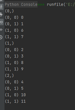
为什么是上面的结果，分析如下？
代码：

i, j = np.nested_iters(a, [[1], [0, 2]], flags=["multi_index"])

的第二个参数：

[[1], [0, 2]]

确定了第1维度(行维度)为父结构，存储在i中；第0维度(列维度)和第2维度为子结构：

由a的数据：

我们可知行维度索引为0,1,2时分别有以下三个子二维矩阵：
行维度索引为0时的子二维矩阵：
$\left[\begin{array}{cc}0& 1\\ 6& 7\end{array}\right]$
行维度索引为1时的子二维矩阵：
$\left[\begin{array}{cc}2& 3\\ 8& 9\end{array}\right]$
行维度索引为2时的子二维矩阵：
$\left[\begin{array}{cc}4& 5\\ 10& 11\end{array}\right]$
如果您对这里的叙述不太理解，可以参考博文：https://blog.csdn.net/wenhao_ir/article/details/125819211

分别遍历这三个子矩阵，便有了上面的运行结果。

05-04-05-flatiter():对数组在一维空间进行迭代

flatiter()

Flat iterator object to iterate over arrays.
示例代码如下：

import numpy as np

A = np.array([[1, 2, 3, 4, 5],
              [6, 7, 8, 9, 10],
              [11, 12, 13, 14, 15]], dtype='int8')

A_flat = A.flat

for item in A_flat:
    print(item)

运行结果如下：


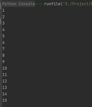
关于代码“A_flat = A.flat”说明一下,flat为ndarray对象的一个属性，该属性用于将数组在一维展平空间进行迭代，详见“02-02-ndarray对象的属性(Attributes)”

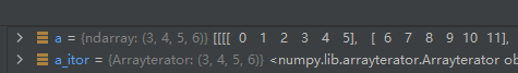
05-04-06-lib.Arrayterator():对数据量大的数组进行优化迭代【每次读取指定大小的连续数据块(缓冲读取)】

lib.Arrayterator(var[, buf_size])

Buffered iterator for big arrays.

这个函数可加快我们对大数据量的数组的迭代处理。
官方文档对其介绍如下：
Arrayterator creates a buffered iterator for reading big arrays in small contiguous blocks. The class is useful for objects stored in the file system. It allows iteration over the object without reading everything in memory; instead, small blocks are read and iterated over.
翻译如下：
Arrayterator创建一个缓冲迭代器，可以通过这个缓冲迭代器以小连续块的形式读取大数据量数组。这种方法对于存储在文件系统中的对象很有效，这样的操作使的迭代操作时无需每次读取存储器中的所有内容，而只需去读取连续小块，然后进行迭代。其第二个参数buf_size可以控制每次读取的大小。
示例代码如下：

import numpy as np

a = np.arange(3 * 4 * 5 * 6).reshape(3, 4, 5, 6)
a_itor = np.lib.Arrayterator(a, 2)

for subarr in a_itor:
    if not subarr.all():
        print(subarr, subarr.shape)

运行结果如下：


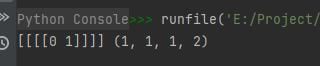
结果分析：
函数all():判断可迭代对象是否所有元素为True，所以语句

    if not subarr.all():
        print(subarr, subarr.shape)

的意思为：
如果subarr中不是所有的元素为True，即有元素为False，那么执行语句：

 print(subarr, subarr.shape)

由于在语句：

a_itor = np.lib.Arrayterator(a, 2)

中我们设置buf_size的大小为2，所以每个迭代对象含2个元素。
根据数组a的数据内容，我们容易判断出第01个迭代对象元素中的两个元素值为0和1，满足条件if not subarr.all()，所有执行了语句 print(subarr, subarr.shape)。嗯，就是这回事。

说白了，这个函数本质上让我们对原矩阵以子矩阵的形式进行快速读取处理。

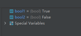
05-04-07-iterable(y):判断对象是否为可迭代对象

iterable(y)

Check whether or not an object can be iterated over.
示例代码如下：

import numpy as np

bool1 = np.iterable([1, 2, 3])
bool2 = np.iterable(2)

运行结果如下：

06-与迭代操作有关的对象和操作(Iterating Over Arrays)

06-01-每次遍历一个元素的迭代操作【利用函数nditer()实现】

函数nditer()已在05-04-01中介绍。

每次遍历一个元素的迭代操作的示例代码如下：

import numpy as np

a = np.arange(6).reshape(2, 3)
for x in np.nditer(a):
    print(x)

运行结果如下：

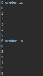
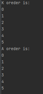
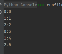
06-02-控制迭代顺序【利用函数nditer()实现】

可以通过设置函数nditer的参数order来控制迭代顺序，实际上是控制是按C语言的存储顺序还是按Fortran的存储顺序，
使用参数 order 控制元素的访问顺序，参数的可选值有C、F、K、A，具体的意义见博文https://blog.csdn.net/wenhao_ir/article/details/125850699

示例代码如下：

import numpy as np

A = np.arange(2*3).reshape(2, 3)

print("C oreder is:")
for x in np.nditer(A, order='C'):  # C表示行优先
    print(x)

print("F oreder is:")
for x in np.nditer(A, order='F'):  # F表示列优先
    print(x)

print("K oreder is:")
for x in np.nditer(A, order='K'):  # 默认值就为K,此种情况下表示“F & C order preserved, otherwise most similar order”
    print(x)

print("A oreder is:")
for x in np.nditer(A, order='A'):  # A在此种情况下表示“F order if input is F and not C, otherwise C order”
    print(x)

运行结果如下：

06-03-通过遍历修改数组值【利用函数nditer()实现】

默认情况下，nditer将输入操作数视为只读对象。为了能够修改数组元素，您必须使用“readwrite”或“writeonly” 每个操作数标志指定读写或只写模式。

然后，nditer 将产生您可以修改的可写缓冲区数组。但是，因为一旦迭代完成，nditer 必须将此缓冲区数据复制回原始数组，因此您必须通过两种方法之一在迭代结束时发出信号。

您可以：

• 使用with语句将 nditer 用作上下文管理器，退出上下文时将写回临时数据。
  关于python中的with…as…语句，可参考博文https://blog.csdn.net/Kwoky/article/details/106682609说白了，with就是其语句块执行完毕后，会关闭或销毁as后的对象。
• 完成迭代后调用迭代器的close方法，这将触发回写。
  一旦调用close或退出其上下文，就不能再迭代 nditer 。
  示例代码如下：

import numpy as np

A = np.arange(6).reshape(2, 3)

with np.nditer(A, op_flags=['readwrite']) as it:
    for x in it:
        x[...] = 2 * x

代码分析：
关于with…as…语句，可参考博文https://blog.csdn.net/Kwoky/article/details/106682609说白了，with就是其语句块执行完毕后，会关闭或销毁as后的对象。
而关于语句x[…] = 2 * x就很不好理解了，只知道a[0, …]的效果和a[0, :]的效果是一样的，只能先理解到这里。

06-04-使用外部循环的external_loop模式加快迭代效率

使用外部循环加快迭代效率。
关于使用外部循环迭代，看下面这篇博文就行了：
https://blog.csdn.net/Shepherdppz/article/details/104255289
鉴于上面博文中末尾提到可以用 np.apply_along_axis()替换external_loop模式下选取行，选取列的迭代操作，并且比所谓的external_loop模式还快，所以这里就不专门写内容研究它了。

值得注意的是：在external_loop模式下，还可以开启缓冲区以增强迭代速度，比如下面的代码：

for x in np.nditer(a, flags=['external_loop','buffered'], order='F'):
    print(x, end=' ')

06-05-跟踪索引操作(类似于枚举化可迭代对象之后的迭代操作)

这个操作类似于枚举化可迭代对象之后的迭代操作，详情见博文 https://blog.csdn.net/wenhao_ir/article/details/125443427
关于nditer()的跟踪索引操作，看下面的几个示例代码和运行结果就很容易明白了：
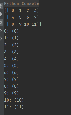
示例代码一：

import numpy as np

# 'c_index' 可以通过 it.index 跟踪C顺序的索引
a = np.arange(12).reshape(3, 4)
print(a)
it = np.nditer(a, flags=['c_index'])
for x in it:
    print("{}: ({})".format(x, it.index))

运行结果：

示例代码二：

import numpy as np

# 'f_index' 可以通过 it.index 跟踪F顺序的索引
a = np.arange(12).reshape(3, 4)
print(a)
it = np.nditer(a, flags=['f_index'])
for x in it:
    print("{}: ({})".format(x, it.index))

运行结果如下：

示例代码三：

import numpy as np

# 'multi_index' 可以通过 it.multi_index 跟踪数组索引
a = np.arange(12).reshape(3, 4)
print(a)
it = np.nditer(a, flags=['multi_index'])
for x in it:
    print("{}: ({})".format(x, it.multi_index))

运行结果如下：

06-06-用特定数据类型进行迭代

有时需要将数组视为与存储时不同的数据类型。例如，一个人可能想要在 64 位浮点数上进行所有计算，即使被操作的数组是 32 位浮点数。除了编写低级 C 代码时，通常最好让迭代器处理复制或缓冲，而不是自己在内部循环中转换数据类型。

有两种机制可以做到这一点，临时副本和缓冲模式。对于临时副本，使用新数据类型制作整个数组的副本，然后在副本中进行迭代。通过在所有迭代完成后更新原始数组的模式允许写访问。临时副本的主要缺点是临时副本可能会消耗大量内存，尤其是在迭代数据类型的项目大小比原始数据类型大的情况下。

缓冲模式缓解了内存使用问题，并且比制作临时副本更便于缓存。除了在迭代器之外一次需要整个数组的特殊情况外，建议使用缓冲而不是临时复制。在 NumPy 中，ufunc 和其他函数使用缓冲来支持灵活的输入，并且内存开销最小。

总结一下：
当需要以其它的数据类型来迭代数组时，有两种方法：

• 临时副本：迭代时，会使用新的数据类型创建数组的副本，然后在副本中完成迭代。但是，这种方法会消耗大量的内存空间。
• 缓冲模式： 使用缓冲来支持灵活输入，内存开销最小。

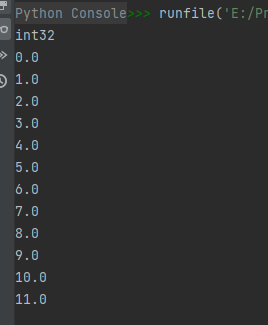
示例代码如下：

import numpy as np

# 临时副本
a = np.arange(12).reshape(3, 4)
print(a.dtype)
it = np.nditer(a, op_flags=['readonly', 'copy'], op_dtypes=[np.float64])
for x in it:
    print("{}".format(x))

import numpy as np

# 缓冲模式
a = np.arange(12).reshape(3, 4)
print(a.dtype)
it = np.nditer(a, flags=['buffered'], op_dtypes=[np.float64])
for x in it:
    print("{}".format(x))

运行结果如下：

06-06-迭代中的广播操作

关于Numpy中的广播操作，可参考博文：
https://blog.csdn.net/Kilig___/article/details/108019155

迭代中的广播操作的示例代码如下：

import numpy as np

a = np.arange(3)
b = np.arange(6).reshape(2, 3)
for x, y in np.nditer([a, b]):
    print("%d:%d" % (x, y))

运行结果如下：

06-07-其它的一些冷门迭代操作

其它的迭代操作还有以下这些：
迭代器分配的输出数组(Iterator-Allocated Output Arrays)、外部结果迭代(Outer Product Iteration)、减少迭代(Reduction Iteration)、将内循环放入Cython(Putting the Inner Loop in Cython)中等，昊虹君觉得这些操作比较冷门，就不一一仔细研究了。
关于Cython，有一篇博文写得不错，大家可以参考下，链接 https://blog.csdn.net/chinesehuazhou2/article/details/125252492

07-ndarray对象的创建

07-01-使用方法numpy.array()和numpy.asarray()创建ndarray对象

可以使用NumPy的方法array()创建一个ndarray对象。

函数array()的语法如下：

numpy.array(object, dtype=None, *, copy=True, order='K', subok=False, ndmin=0, like=None)

函数array()的官方文档链接：https://numpy.org/doc/stable/reference/generated/numpy.array.html?highlight=array#numpy.array

参数意义如下：
object—数组型对象，要求对象的方法__array__能返回一个数组或任何序列(可嵌套)。如果object是个标量，那么object是0维的。这个参数最常见的对象是列表对象。列表对象中就有方法__array__。
dtype—数据类型，可选参数。如果这个值没有指定，那么函数array()会选用能满足存储要求而占用空间最小的数据类型。
copy—是否复制object的标志，也是可选参数。这个参数用于配合参数order来控制矩阵数据的内存布局，详情见对order参数的介绍。

order—指定矩阵数据的内存布局，默认值为K。该参数和参数copy配合使用来控制矩阵数据的内存布局，详情见下表：

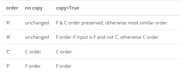
表中的C order代表C语言的数据存储结构，F代表Fortrany语言的数据存储结构。
copy的默认值为True，order的默认值为K，从上表来看，这样的默认组合意味着F和C的数据存储被保留，而对于别的存储数据也会尽量保持相似。
subok—如果为True，则返回的子类对象矩阵会被存储，否则返回的矩阵将被强制为基类矩阵对象（默认）。
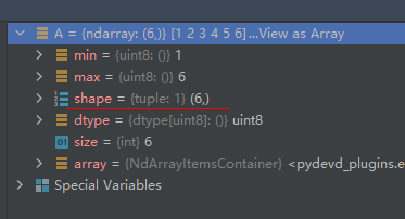
ndmin—矩阵的最小维度，一般这个值都不填，而是自己填写数据格式控制维度。示例如下：

A = np.array([1, 2, 3, 4, 5, 6], dtype='uint8')

运行结果如下：

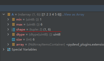
A = np.array([1, 2, 3, 4, 5, 6], dtype='uint8', ndmin=2)

运行结果如下：

A = np.array([1, 2, 3, 4, 5, 6], dtype='uint8', ndmin=3)

运行结果如下：

like—这个参数用于控制生成的矩阵是否为NumPy型矩阵，如果要生成别的类型的矩阵，那么like参数对象应该满足__array_function__ 协议。

方法numpy.array()完整的示例代码如下：

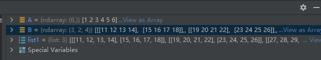
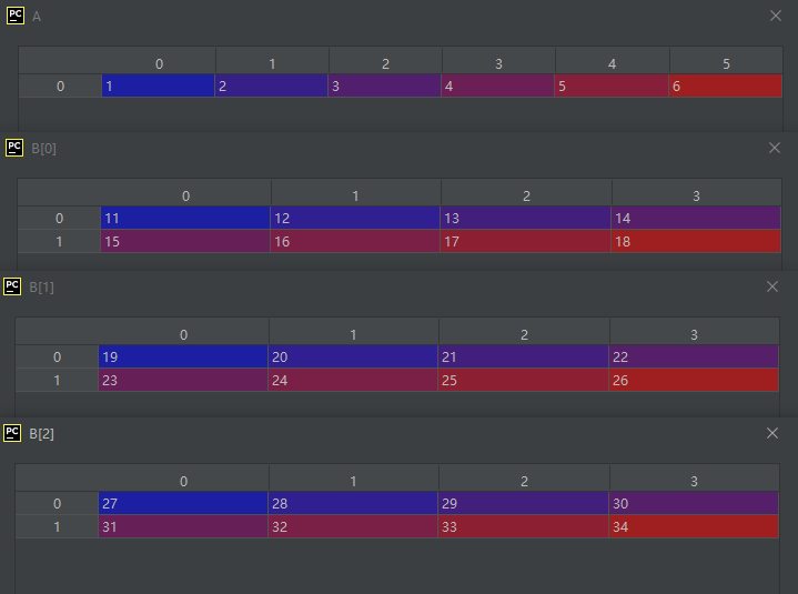
import numpy as np

A = np.array([1, 2, 3, 4, 5, 6], dtype='uint8')

list1 = [[[11, 12, 13, 14],
         [15, 16, 17, 18]],
         [[19, 20, 21, 22],
         [23, 24, 25, 26]],
         [[27, 28, 29, 30],
         [31, 32, 33, 34]]]

B = np.array(list1)

运行结果如下：


方法numpy.asarray()与方法numpy.array()功能相同，不同之处在于方法numpy.asarray()比方法numpy.array()的参数少三个。

方法numpy.array()的语法如下：

numpy.array(object, dtype=None, *, copy=True, order='K', subok=False, ndmin=0, like=None)

方法numpy.asarray()的语法如下：

numpy.asarray(a, dtype=None, order=None, *, like=None)

因为使用方法一样，所以就不给示例代码了。只要补充说一下“as”的来历，asarray()实际上可看成是把列表、元组等转换为ndarray对象，所以“as”是可理解为转换的意思，类似的函数有astype()，详情见 https://blog.csdn.net/wenhao_ir/article/details/124399693

07-02-使用方法numpy.empty()创建一个指定形状（shape）、数据类型（dtype）且未初始化的ndarray对象(矩阵)

语法如下：

numpy.empty(shape, dtype = float, order = 'C')

第三个参数有"C"和"F"两个选项，即在计算机内存中的存储元素的顺序。实质上就是C语言和Fortrany语言的存储顺序。
示例代码如下：

import numpy as np

A = np.empty([3, 2], dtype=int)

运行结果如下：

从运行结果可见，由于数据的值未初始化，所以值是不定义的。

07-03-使用方法numpy.zeros()创建指定大小,元素值为0的ndarray对象(矩阵)

语法如下：

numpy.zeros(shape, dtype = float, order = 'C')

示例代码如下：

import numpy as np

A = np.zeros([3, 2])
B = np.zeros([3, 2], dtype=int)

运行结果如下：

可见，没有没有指定类型，默认的确为float型。

07-04-使用方法numpy.ones()创建指定大小,元素值为1的ndarray对象(矩阵)

语法如下：

numpy.ones(shape, dtype = None, order = 'C')

示例代码如下：

import numpy as np

A = np.ones([3, 2])
B = np.ones([3, 2], dtype=int)

运行结果如下：

07-05-使用方法numpy.frombuffer()从buffer读取数据生成一维矩阵

这个方法不常用，所以只给出语法和帮助文档链接：

语法如下：

numpy.frombuffer(buffer, dtype=float, count=- 1, offset=0, *, like=None)

文档链接：
https://numpy.org/doc/stable/reference/generated/numpy.frombuffer.html
https://www.runoob.com/numpy/numpy-array-from-existing-data.html

07-06-使用方法numpy.fromiter()从可迭代对象生成一维矩阵

语法如下：

numpy.fromiter(iter, dtype, count=- 1, *, like=None)

文档链接：
https://numpy.org/doc/stable/reference/generated/numpy.fromiter.html
https://www.runoob.com/numpy/numpy-array-from-existing-data.html

07-07-使用方法numpy.arange()从数值范围创建矩阵

语法如下：

numpy.arange([start, ]stop, [step, ]dtype=None, *, like=None)

根据 start 与 stop 指定的范围以及 step 设定的步长，生成一个 ndarray。
注意，数值范围区间为[start, stop)，即左开右闭区间。

07-08-From shape or value【根据array的形状和值创建ndarray对象、复制别的array的形状创建具有一定值的ndarray对象】

• empty(shape[, dtype, order, like])
  Return a new array of given shape and type, without initializing entries.

• empty_like(prototype[, dtype, order, subok, …])
  Return a new array with the same shape and type as a given array.

• eye(N[, M, k, dtype, order, like])
  Return a 2-D array with ones on the diagonal and zeros elsewhere.

• identity(n[, dtype, like])
  Return the identity array.(返回对角矩阵)

• ones(shape[, dtype, order, like])
  Return a new array of given shape and type, filled with ones.

• ones_like(a[, dtype, order, subok, shape])
  Return an array of ones with the same shape and type as a given array.

• zeros(shape[, dtype, order, like])
  Return a new array of given shape and type, filled with zeros.

• zeros_like(a[, dtype, order, subok, shape])
  Return an array of zeros with the same shape and type as a given array.

• full(shape, fill_value[, dtype, order, like])
  Return a new array of given shape and type, filled with fill_value.

• full_like(a, fill_value[, dtype, order, …])
  Return a full array with the same shape and type as a given array.

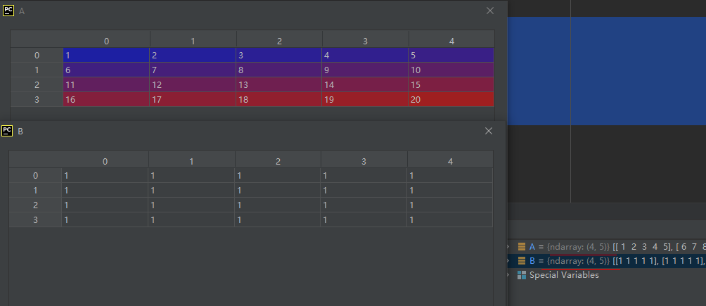
上面以“_like”结尾的函数，看下面的示例就清楚用法了：

import numpy as np

A = np.array([[1, 2, 3, 4, 5],
              [6, 7, 8, 9, 10],
              [11, 12, 13, 14, 15],
              [16, 17, 18, 19, 20]], dtype='int8')

B = np.ones_like(A)

07-09-From existing data(从已有数据创建array)

• array(object[, dtype, copy, order, subok, …])
  Create an array.
  函数array()的语法如下：

numpy.array(object, dtype=None, *, copy=True, order='K', subok=False, ndmin=0, like=None)

函数array()的官方文档链接：https://numpy.org/doc/stable/reference/generated/numpy.array.html?highlight=array#numpy.array

参数意义如下：
object—数组型对象，要求对象的方法__array__能返回一个数组或任何序列(可嵌套)。如果object是个标量，那么object是0维的。这个参数最常见的对象是列表对象。列表对象中就有方法__array__。
dtype—数据类型，可选参数。如果这个值没有指定，那么函数array()会选用能满足存储要求而占用空间最小的数据类型。
copy—是否复制object的标志，也是可选参数。这个参数用于配合参数order来控制矩阵数据的内存布局，详情见对order参数的介绍。

order—指定矩阵数据的内存布局，默认值为K。该参数和参数copy配合使用来控制矩阵数据的内存布局，详情见下表：

表中的C order代表C语言的数据存储结构，F代表Fortrany语言的数据存储结构。
copy的默认值为True，order的默认值为K，从上表来看，这样的默认组合意味着F和C的数据存储被保留，而对于别的存储数据也会尽量保持相似。
subok—如果为True，则返回的子类对象矩阵会被存储，否则返回的矩阵将被强制为基类矩阵对象（默认）。
ndmin—矩阵的最小维度，一般这个值都不填，而是自己填写数据格式控制维度。示例如下：

A = np.array([1, 2, 3, 4, 5, 6], dtype='uint8')

运行结果如下：

A = np.array([1, 2, 3, 4, 5, 6], dtype='uint8', ndmin=2)

运行结果如下：

A = np.array([1, 2, 3, 4, 5, 6], dtype='uint8', ndmin=3)

运行结果如下：

like—这个参数用于控制生成的矩阵是否为NumPy型矩阵，如果要生成别的类型的矩阵，那么like参数对象应该满足__array_function__ 协议。

方法numpy.array()完整的示例代码如下：

import numpy as np

A = np.array([1, 2, 3, 4, 5, 6], dtype='uint8')

list1 = [[[11, 12, 13, 14],
         [15, 16, 17, 18]],
         [[19, 20, 21, 22],
         [23, 24, 25, 26]],
         [[27, 28, 29, 30],
         [31, 32, 33, 34]]]

B = np.array(list1)

运行结果如下：


方法numpy.asarray()与方法numpy.array()功能相同，第一个不同之处在于方法numpy.asarray()比方法numpy.array()的参数少三个。

方法numpy.array()的语法如下：

numpy.array(object, dtype=None, *, copy=True, order='K', subok=False, ndmin=0, like=None)

方法numpy.asarray()的语法如下：

numpy.asarray(a, dtype=None, order=None, *, like=None)

因为使用方法一样，所以就不给示例代码了。只要补充说一下“as”的来历，asarray()实际上可看成是把列表、元组等转换为ndarray对象，所以“as”是可理解为转换的意思，类似的函数有astype()，详情见 https://blog.csdn.net/wenhao_ir/article/details/124399693
第二个不同之处是当第一个参数为ndarray对象时，array()为深拷贝，asarray()为浅拷贝，详情见博文 https://blog.csdn.net/m0_37617773/article/details/121611977

• asarray(a[, dtype, order, like])
  Convert the input to an array.

• asanyarray(a[, dtype, order, like])
  Convert the input to an ndarray, but pass ndarray subclasses through.
  博主注：这个函数的用法见博文 https://blog.csdn.net/m0_37617773/article/details/121611977(注意：这篇博文最后给了示例代码的)
  要想深刻理解asanyarray(),可以参见对“Standard array subclasses”的介绍：
  链接：
  https://numpy.org/doc/stable/reference/arrays.classes.html
  原文：
  Note that asarray always returns the base-class ndarray. If you are confident that your use of the array object can handle any subclass of an ndarray, then asanyarray can be used to allow subclasses to propagate more cleanly through your subroutine. In principal a subclass could redefine any aspect of the array and therefore, under strict guidelines, asanyarray would rarely be useful. However, most subclasses of the array object will not redefine certain aspects of the array object such as the buffer interface, or the attributes of the array. One important example, however, of why your subroutine may not be able to handle an arbitrary subclass of an array is that matrices redefine the “” operator to be matrix-multiplication, rather than element-by-element multiplication.*
  翻译：
  注意，asarray始终返回基类ndarray。如果您确信使用array对象可以处理ndarray的任何子类，那么可以使用asanyarray允许子类通过子例程更干净地传播。原则上，子类可以重新定义数组的任何方面，因此，在严格的准则下，asanyarray很少有用。然而，数组对象的大多数子类不会重新定义数组对象的某些方面，例如缓冲区接口或数组的属性。然而，一个重要的例子是，为什么子例程可能无法处理数组的任意子类，矩阵将“*”运算符重新定义为矩阵乘法，而不是逐元素乘法。

• ascontiguousarray(a[, dtype, like])
  Return a contiguous array (ndim >= 1) in memory (C order).

• asmatrix(data[, dtype])
  Interpret the input as a matrix.
  Unlike matrix, asmatrix does not make a copy if the input is already a matrix or an ndarray.
  理解上面这段话时要注意：numpy是一个类，其主要对象为ndarray对象，matrix为numpy的标准子类，其对象为matrix。

• copy(a[, order, subok])
  Return an array copy of the given object.

• frombuffer(buffer[, dtype, count, offset, like])
  Interpret a buffer as a 1-dimensional array.

• from_dlpack(x, /)
  Create a NumPy array from an object implementing the dlpack protocol.

• fromfile(file[, dtype, count, sep, offset, like])
  Construct an array from data in a text or binary file.
  可见，Numpy库在创建array时还能从文件读取数据哦，以后可以试一试。以后要用的时候也同时考虑下loadtxt()

• fromfunction(function, shape, *[, dtype, like])
  Construct an array by executing a function over each coordinate.
  还能通过调用函数生成？是的，常见的就是匿名函数嘛~善于运用的话，可以节省不少代码哦，示例如下：
  
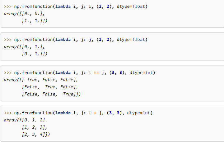
  上面的示例的链接：
  https://numpy.org/doc/stable/reference/generated/numpy.fromfunction.html#numpy.fromfunction

• fromiter(iter, dtype[, count, like])
  Create a new 1-dimensional array from an iterable object.

• fromstring(string[, dtype, count, like])
  A new 1-D array initialized from text data in a string.
  不错哦，还能把字符或字符串转为数字，Python实在是太强大了。这在C++中就得用操作了，而且不是一句代码能搞定的。

import numpy as np

A = np.fromstring('1 2', dtype=int, sep=' ')

运行结果如下：

• loadtxt(fname[, dtype, comments, delimiter, …])
  Load data from a text file.
  这也是从文件读取数据，以后要用的时候也同时考虑下fromfile()

08-ndarray的属性(维度、形状、元素个数、数据类型、每个元素占用的内存空间、内存布局、数据的实部、数据的虚部)

关于ndarray的属性，详见博文 https://blog.csdn.net/wenhao_ir/article/details/124416798 的第8点。

09-Numpy的数据类型

关于Numpy的数据类型的详情，见博文：
https://blog.csdn.net/wenhao_ir/article/details/124409146

10-Standard array subclasses(标准array 子类)

10-01-Matrix objects

官方文档首先就说了不建议使用它，原因如下：
强烈建议不要使用矩阵子类。如下所述，这使得编写一致处理矩阵和正则数组的函数非常困难。目前，它们主要用于与scipy交互。然而，我们希望为这种使用提供一种替代方法，并最终删除矩阵子类。
可见，在Numpy中存在这个主要是为了与scipy库进行交互，最终，Numpy官方希望能找到一种方法，使得矩阵子类可以被彻底淘汰。

10-02-Memory-mapped file arrays

内存映射文件对于读取和/或修改具有规则布局的大文件的小段非常有用，而无需将整个文件读入内存。ndarray的一个简单子类使用内存映射文件作为数组的数据缓冲区。对于小文件，将整个文件读入内存的开销通常不太大，但是对于大文件，使用内存映射可以节省大量资源。
可见：这个子类是针对大文件操作时节省内存空间的操作。

10-03-Character arrays (numpy.char)

这是字符型子类，也就是说里面的元素类型为字符。

10-04-Record arrays (numpy.rec)

numpy.rec is the preferred alias for numpy.core.records.

numpy.record类的对象有点类似于结构体化的array，它是Numpy的标准子类，官方文档对其描述如下：
A data-type scalar that allows field access as attribute lookup.
翻译如下：
允许作为属性查找进行字段访问的数据类型标量
官方文档链接：https://numpy.org/doc/stable/reference/generated/numpy.record.html
可以通过下面这篇文章：
https://cloud.tencent.com/developer/article/1837178（搜索关键词“结构化数组只能通过index来访问”）
对其有个清晰的认识。

11-Constants(Numpy库中的常量)

数学库怎么离得了数学常量，Numpy库自然也有。

• numpy.inf–正无穷大。
• numpy.Inf—正无穷大，官方建议用"inf"表示正无穷大。
• numpy.Infinity—也是正无穷大，官方建议用"inf"表示正无穷大。
• numpy.PINF—也是正无穷大，官方建议用"inf"表示正无穷大。
• numpy.infty—也是正无穷大，官方建议用"inf"表示正无穷大。
• numpy.NINF—负无穷大
• numpy.nan—Not a Number，表示未定义或不可表示的值。常在浮点数运算中使用。首次引入NaN的是1985年的IEEE 754浮点数标准。
• numpy.NAN—同nan，官方建议用nan。
• numpy.NaN—同numpy.NAN。
• numpy.NZERO—negative zero，即负0值，负0值怎么理解？请联系高等数学中极限的概念理解。
• numpy.PZERO—也是负0值。
• numpy.e–自然常数e。
• numpy.euler_gamma—欧拉常数(Euler-Mascheroni constant)
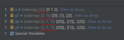
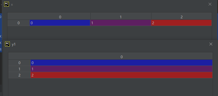
• numpy.newaxis—表示某个维度为空，示例代码如下：

import numpy as np

x = np.arange(3)
y1 = x[:, np.newaxis]
y2 = x[:, np.newaxis, np.newaxis]
y3 = y1[:, np.newaxis]

运行结果如下：

12-Universal functions (ufunc)【逐元素操作类】

Universal functions简称为ufunc，直译为通用函数，根据官方文档的解释，这类函数会对array中的所有元素进行逐元素操作。

在Python中由ufunc类实现这些逐元素操作方法。

NumPy内置的许多ufunc函数都是用C语言实现的，因此它们的计算速度非常快。

12-01-ufunc类的Attributes(属性)

上面这个截图的官方链接：
https://numpy.org/doc/stable/reference/ufuncs.html#attributes

12-02-ufunc类的Methods(方法)

以上这些方法都是与某种具体的运算相结合实现某个具体的功能。也就是说这些方法被具体的运算类继承，看下面的这句示例代码你就明白了：

np.add.accumulate([2, 3, 5])

显然，通过上面的示例语句我们可以知道，类add继续了类ufunc的方法accumulate()

12-02-01-ufunc.reduce()【减少array的维度】

ufunc.reduce(array[, axis, dtype, out, ...])

这个方法用于减少array的维度。

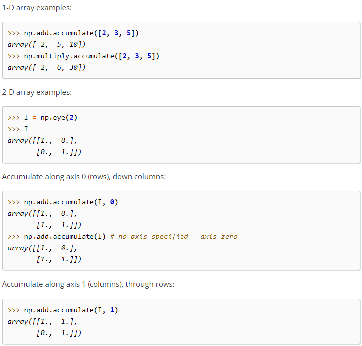
12-02-02-ufunc.accumulat()【累加各种运算结果】

ufunc.accumulate(array[, axis, dtype, out])

这个方法用于对各种运算结果进行累加，示例代码如下：

12-02-03-ufunc.reduceat()【分片合并array元素】

ufunc.reduceat(array, indices[, axis, ...])

这个方法用于分片合并array元素。
示例如下：

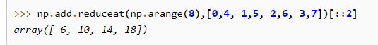
上面截图中的第一个元素来历：
6 = 0 + 1 + 2 +3 = 6；
第二个元素来历：
10 = 1+2+3+4 = 10;
…

12-02-04-ufunc.outer【a中的每一个元素,依次对b中的每个元素进行运算】

ufunc.outer(a, b, /, **kwargs)

a中每一个元素，依次对b中的每个元素进行运算。


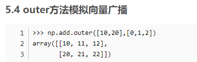
上面的截图来自于博文：
https://blog.csdn.net/hustlei/article/details/122011299

12-02-04-ufunc.at()【逐元素做某种操作】

语法如下：

ufunc.at(a, indices[, b])

12-03-适用于ufunc类的数学操作

• add(x1, x2, /[, out, where, casting, order, …])
  Add arguments element-wise.

• subtract(x1, x2, /[, out, where, casting, …])
  Subtract arguments, element-wise.

• multiply(x1, x2, /[, out, where, casting, …])
  Multiply arguments element-wise.

• matmul(x1, x2, /[, out, casting, order, …])
  Matrix product of two arrays.

• divide(x1, x2, /[, out, where, casting, …])
  Divide arguments element-wise.

• logaddexp(x1, x2, /[, out, where, casting, …])
  Logarithm of the sum of exponentiations of the inputs.

• logaddexp2(x1, x2, /[, out, where, casting, …])
  Logarithm of the sum of exponentiations of the inputs in base-2.

• true_divide(x1, x2, /[, out, where, …])
  Divide arguments element-wise.

• floor_divide(x1, x2, /[, out, where, …])
  Return the largest integer smaller or equal to the division of the inputs.

• negative(x, /[, out, where, casting, order, …])
  Numerical negative, element-wise.

• positive(x, /[, out, where, casting, order, …])
  Numerical positive, element-wise.

• power(x1, x2, /[, out, where, casting, …])
  First array elements raised to powers from second array, element-wise.

• float_power(x1, x2, /[, out, where, …])
  First array elements raised to powers from second array, element-wise.

• remainder(x1, x2, /[, out, where, casting, …])
  Returns the element-wise remainder of division.

• mod(x1, x2, /[, out, where, casting, order, …])
  Returns the element-wise remainder of division.

• fmod(x1, x2, /[, out, where, casting, …])
  Returns the element-wise remainder of division.

• divmod(x1, x2[, out1, out2], / [[, out, …])
  Return element-wise quotient and remainder simultaneously.

• absolute(x, /[, out, where, casting, order, …])
  Calculate the absolute value element-wise.

• fabs(x, /[, out, where, casting, order, …])
  Compute the absolute values element-wise.

• rint(x, /[, out, where, casting, order, …])
  Round elements of the array to the nearest integer.

• sign(x, /[, out, where, casting, order, …])
  Returns an element-wise indication of the sign of a number.

• heaviside(x1, x2, /[, out, where, casting, …])
  Compute the Heaviside step function.

• conj(x, /[, out, where, casting, order, …])
  Return the complex conjugate, element-wise.

• conjugate(x, /[, out, where, casting, …])
  Return the complex conjugate, element-wise.

• exp(x, /[, out, where, casting, order, …])
  Calculate the exponential of all elements in the input array.

• exp2(x, /[, out, where, casting, order, …])
  Calculate 2**p for all p in the input array.

• log(x, /[, out, where, casting, order, …])
  Natural logarithm, element-wise.

• log2(x, /[, out, where, casting, order, …])
  Base-2 logarithm of x.

• log10(x, /[, out, where, casting, order, …])
  Return the base 10 logarithm of the input array, element-wise.

• expm1(x, /[, out, where, casting, order, …])
  Calculate exp(x) - 1 for all elements in the array.

• log1p(x, /[, out, where, casting, order, …])
  Return the natural logarithm of one plus the input array, element-wise.

• sqrt(x, /[, out, where, casting, order, …])
  Return the non-negative square-root of an array, element-wise.

• square(x, /[, out, where, casting, order, …])
  Return the element-wise square of the input.

• cbrt(x, /[, out, where, casting, order, …])
  Return the cube-root of an array, element-wise.

• reciprocal(x, /[, out, where, casting, …])
  Return the reciprocal of the argument, element-wise.

• gcd(x1, x2, /[, out, where, casting, order, …])
  Returns the greatest common divisor of |x1| and |x2|

• lcm(x1, x2, /[, out, where, casting, order, …])
  Returns the lowest common multiple of |x1| and |x2|
  上面这些数学运算大部分通过学习Python和C++/C的math库已经知道其作用了，详情见：
  https://blog.csdn.net/wenhao_ir/article/details/125607783
  https://blog.csdn.net/wenhao_ir/article/details/125639428
  只说下自己觉得需要说下的：
  rint()—Round elements of the array to the nearest integer.可见这个实际上是math库中的round()
  heavisidet()----单位阶跃函数的值,单位阶跃函数又称赫维赛德阶跃( Heaviside step function )函数。
  reciprocal—倒数
  gcd()—最大公约数,greatest common divisor简写为gcd
  lcm()—最小公倍数,最小公倍数

12-04-适用于ufunc类的三角函数

• sin(x, /[, out, where, casting, order, …])
  Trigonometric sine, element-wise.

• cos(x, /[, out, where, casting, order, …])
  Cosine element-wise.

• tan(x, /[, out, where, casting, order, …])
  Compute tangent element-wise.

• arcsin(x, /[, out, where, casting, order, …])
  Inverse sine, element-wise.

• arccos(x, /[, out, where, casting, order, …])
  Trigonometric inverse cosine, element-wise.

• arctan(x, /[, out, where, casting, order, …])
  Trigonometric inverse tangent, element-wise.

• arctan2(x1, x2, /[, out, where, casting, …])
  Element-wise arc tangent of x1/x2 choosing the quadrant correctly.

• hypot(x1, x2, /[, out, where, casting, …])
  Given the “legs” of a right triangle, return its hypotenuse.

• sinh(x, /[, out, where, casting, order, …])
  Hyperbolic sine, element-wise.

• cosh(x, /[, out, where, casting, order, …])
  Hyperbolic cosine, element-wise.

• tanh(x, /[, out, where, casting, order, …])
  Compute hyperbolic tangent element-wise.

• arcsinh(x, /[, out, where, casting, order, …])
  Inverse hyperbolic sine element-wise.

• arccosh(x, /[, out, where, casting, order, …])
  Inverse hyperbolic cosine, element-wise.

• arctanh(x, /[, out, where, casting, order, …])
  Inverse hyperbolic tangent element-wise.

• degrees(x, /[, out, where, casting, order, …])
  Convert angles from radians to degrees.

• radians(x, /[, out, where, casting, order, …])
  Convert angles from degrees to radians.

• deg2rad(x, /[, out, where, casting, order, …])
  Convert angles from degrees to radians.

• rad2deg(x, /[, out, where, casting, order, …])
  Convert angles from radians to degrees.

上面这些三角函数运算大部分通过学习Python和C++/C的math库已经知道其作用了，详情见：
https://blog.csdn.net/wenhao_ir/article/details/125607783
https://blog.csdn.net/wenhao_ir/article/details/125639428
只说下自己觉得需要说下的：
hypot–计算三角形的斜边长。

12-05-适用于ufunc类的位运算函数

• bitwise_and(x1, x2, /[, out, where, …])
  Compute the bit-wise AND of two arrays element-wise.

• bitwise_or(x1, x2, /[, out, where, casting, …])
  Compute the bit-wise OR of two arrays element-wise.

• bitwise_xor(x1, x2, /[, out, where, …])
  Compute the bit-wise XOR of two arrays element-wise.

• invert(x, /[, out, where, casting, order, …])
  Compute bit-wise inversion, or bit-wise NOT, element-wise.

• left_shift(x1, x2, /[, out, where, casting, …])
  Shift the bits of an integer to the left.

• right_shift(x1, x2, /[, out, where, …])
  Shift the bits of an integer to the right.

没啥好补充说的，就是位运算的那几种运算，只是注意Numpy库还为我们提供了左移运算和右移运算。

12-06-适用于ufunc类的比较运算和逻辑运算函数

• greater(x1, x2, /[, out, where, casting, …])
  Return the truth value of (x1 > x2) element-wise.

• greater_equal(x1, x2, /[, out, where, …])
  Return the truth value of (x1 >= x2) element-wise.

• less(x1, x2, /[, out, where, casting, …])
  Return the truth value of (x1 < x2) element-wise.

• less_equal(x1, x2, /[, out, where, casting, …])
  Return the truth value of (x1 <= x2) element-wise.

• not_equal(x1, x2, /[, out, where, casting, …])
  Return (x1 != x2) element-wise.

• equal(x1, x2, /[, out, where, casting, …])
  Return (x1 == x2) element-wise.

• logical_and(x1, x2, /[, out, where, …])
  Compute the truth value of x1 AND x2 element-wise.

• logical_or(x1, x2, /[, out, where, casting, …])
  Compute the truth value of x1 OR x2 element-wise.

• logical_xor(x1, x2, /[, out, where, …])
  Compute the truth value of x1 XOR x2, element-wise.

• logical_not(x, /[, out, where, casting, …])
  Compute the truth value of NOT x element-wise.

12-07-适用于ufunc类的浮点数运算函数

-isfinite(x, /[, out, where, casting, order, …])
Test element-wise for finiteness (not infinity and not Not a Number).

-isinf(x, /[, out, where, casting, order, …])
Test element-wise for positive or negative infinity.

-isnan(x, /[, out, where, casting, order, …])
Test element-wise for NaN and return result as a boolean array.

-isnat(x, /[, out, where, casting, order, …])
Test element-wise for NaT (not a time) and return result as a boolean array.

-fabs(x, /[, out, where, casting, order, …])
Compute the absolute values element-wise.

-signbit(x, /[, out, where, casting, order, …])
Returns element-wise True where signbit is set (less than zero).

-copysign(x1, x2, /[, out, where, casting, …])
Change the sign of x1 to that of x2, element-wise.

-nextafter(x1, x2, /[, out, where, casting, …])
Return the next floating-point value after x1 towards x2, element-wise.

-spacing(x, /[, out, where, casting, order, …])
Return the distance between x and the nearest adjacent number.

-modf(x[, out1, out2], / [[, out, where, …])
Return the fractional and integral parts of an array, element-wise.

-ldexp(x1, x2, /[, out, where, casting, …])
Returns x1 * 2**x2, element-wise.

-frexp(x[, out1, out2], / [[, out, where, …])
Decompose the elements of x into mantissa and twos exponent.

-fmod(x1, x2, /[, out, where, casting, …])
Returns the element-wise remainder of division.

-floor(x, /[, out, where, casting, order, …])
Return the floor of the input, element-wise.

-ceil(x, /[, out, where, casting, order, …])
Return the ceiling of the input, element-wise.

-trunc(x, /[, out, where, casting, order, …])
Return the truncated value of the input, element-wise.
上面这些数学运算大部分通过学习Python和C++/C的math库已经知道其作用了，详情见：
https://blog.csdn.net/wenhao_ir/article/details/125607783
https://blog.csdn.net/wenhao_ir/article/details/125639428
只说下自己觉得需要说下的：
spacing()—求浮点数相对精度，相当于MATLAB中的函数eps，所以搜索“matlab eps”就可以找到它的用法了。

13-Routines(常用操作及相关的方法、函数)

这一部分内容是整个Numpy库帮助文档的核心，所以必须认真、仔细读一遍。

............................

写到这里，昊虹君抬头看了一下，这库的内容还很多，实在是没时间去一一深入了解了，实际上这样的了解也是比较枯燥的。
所以暂时就先写到这里，以后再慢慢补充吧！
有一个重要的心得那就是：要善于用英文作为关键词去搜索扩展库的官方帮助文档。