机器学习笔记 - 时间序列的混合模型

一、组成和残差

线性回归擅长推断趋势，但无法学习交互作用。 XGBoost 擅长学习交互，但无法推断趋势。在本课中，我们将学习如何创建“混合”预测器，将互补的学习算法结合起来，让一个的优势弥补另一个的弱点。

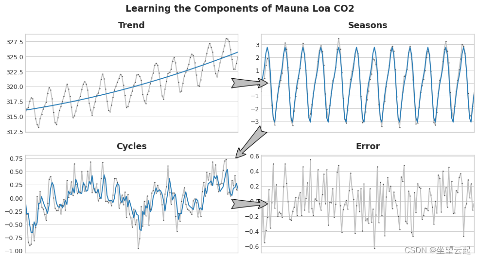
为了设计出有效的混合模型，我们需要更好地理解时间序列是如何构建的。到目前为止，我们已经研究了三种依赖模式：趋势、季节和周期。许多时间序列可以通过仅由这三个组件加上一些本质上不可预测的完全随机误差的加法模型来密切描述：

series = trend + seasons + cycles + error

这个模型中的每一项我们都可以称为时间序列的一个组成部分。

模型的残差是模型训练的目标与模型做出的预测之间的差异——换句话说，就是实际曲线和拟合曲线之间的差异。根据特征绘制残差，你会得到目标的“剩余”部分，或者模型未能从该特征中了解目标的内容。

上图左侧是隧道交通系列的一部分和第 3 课中的趋势-季节性曲线。减去拟合曲线后，残差在右侧。残差包含趋势季节性模型没有学习的隧道交通中的所有内容。

我们可以将学习时间序列的组成部分想象为一个迭代过程：首先学习趋势并将其从序列中减去，然后从去趋势的残差中学习季节性并减去季节，然后学习周期并减去周期，最后只剩下不可预知的错误。

逐步学习 Mauna Loa CO2 的组成。从其系列中减去拟合曲线（蓝色）以获得下一步中的系列。

将我们学到的所有组件加在一起，我们就得到了完整的模型。如果您在一组完整的特征建模趋势、季节和周期上对其进行训练，这基本上就是线性回归会做的事情。

二、残差混合预测

在之前我们使用单一算法（线性回归）一次学习所有组件。但也可以对某些组件使用一种算法，而对其余组件使用另一种算法。这样，我们总是可以为每个组件选择最佳算法。为此，我们使用一种算法来拟合原始序列，然后使用第二种算法来拟合残差序列。

详细来说，流程是这样的：

# 1. 使用第一个模型进行训练和预测
model_1.fit(X_train_1, y_train)
y_pred_1 = model_1.predict(X_train)

# 2. 使用残差的第二个模型进行训练和预测
model_2.fit(X_train_2, y_train - y_pred_1)
y_pred_2 = model_2.predict(X_train_2)

# 3. 添加以获得整体预测
y_pred = y_pred_1 + y_pred_2

根据我们希望每个模型学习的内容，我们通常希望使用不同的特征集（上面的 X_train_1 和 X_train_2）。例如，如果我们使用第一个模型来学习趋势，我们通常不需要第二个模型的趋势特征。

虽然可以使用两个以上的模型，但实际上它似乎并不是特别有用。事实上，构建混合模型最常见的策略就是我们刚刚描述的：一个简单（通常是线性）学习算法，然后是一个复杂的非线性学习器，如 GBDT 或深度神经网络，简单模型通常设计为后面强大算法的“助手”。

1、设计混合

还有很多方法可以组合机器学习模型。然而，成功地组合模型需要我们更深入地研究这些算法是如何运作的。

回归算法通常可以通过两种方式进行预测：通过转换特征或转换目标。特征转换算法学习一些将特征作为输入的数学函数，然后将它们组合和转换以产生与训练集中的目标值匹配的输出。线性回归和神经网络就是这种类型。

目标变换算法使用这些特征对训练集中的目标值进行分组，并通过对组中的值进行平均来进行预测；一组特征只是指示要平均哪个组。决策树和最近邻就是这种类型。

重要的是：特征转换器通常可以在给定适当特征作为输入的情况下将目标值外推到训练集之外，但目标转换器的预测将始终限制在训练集的范围内。如果时间虚拟变量继续计算时间步长，则线性回归继续绘制趋势线。给定相同的假定时间，决策树将永远预测训练数据的最后一步所指示的趋势。决策树无法推断趋势。随机森林和梯度提升决策树（如 XGBoost）是决策树的集合，因此它们也无法推断趋势。

这种差异是混合设计的动机：使用线性回归来推断趋势，转换目标以消除趋势，并将 XGBoost 应用于去趋势的残差。要混合神经网络（特征转换器），您可以将另一个模型的预测作为特征包含在内，然后神经网络会将其作为其自身预测的一部分。对残差的拟合方法其实和梯度提升算法使用的方法是一样的，所以我们称这些提升混合；使用预测作为特征的方法称为“堆叠”，因此我们将这些称为堆叠混合。

三、示例 - 零售额

零售销售数据集包含人口普查局收集的 1992 年至 2019 年各个零售行业的月度销售数据。我们的目标是根据早些年的销售额预测 2016-2019 年的销售额。除了创建线性回归 + XGBoost 混合，我们还将了解如何设置用于 XGBoost 的时间序列数据集。

from pathlib import Path
from warnings import simplefilter

import matplotlib.pyplot as plt
import pandas as pd
from sklearn.linear_model import LinearRegression
from sklearn.model_selection import train_test_split
from statsmodels.tsa.deterministic import CalendarFourier, DeterministicProcess
from xgboost import XGBRegressor


simplefilter("ignore")

# Set Matplotlib defaults
plt.style.use("seaborn-whitegrid")
plt.rc(
    "figure",
    autolayout=True,
    figsize=(11, 4),
    titlesize=18,
    titleweight='bold',
)
plt.rc(
    "axes",
    labelweight="bold",
    labelsize="large",
    titleweight="bold",
    titlesize=16,
    titlepad=10,
)
plot_params = dict(
    color="0.75",
    style=".-",
    markeredgecolor="0.25",
    markerfacecolor="0.25",
)

data_dir = Path("../input/ts-course-data/")
industries = ["BuildingMaterials", "FoodAndBeverage"]
retail = pd.read_csv(
    data_dir / "us-retail-sales.csv",
    usecols=['Month'] + industries,
    parse_dates=['Month'],
    index_col='Month',
).to_period('D').reindex(columns=industries)
retail = pd.concat({'Sales': retail}, names=[None, 'Industries'], axis=1)

retail.head()

Industries	Sales
Month	BuildingMaterials	FoodAndBeverage
1992-01-01	8964	29589
1992-02-01	9023	28570
1992-03-01	10608	29682
1992-04-01	11630	30228
1992-05-01	12327	31677

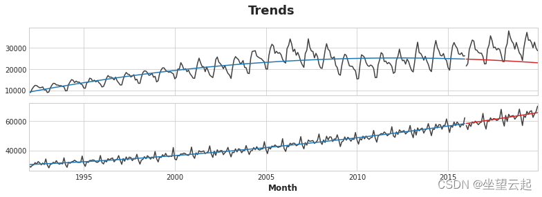
首先让我们使用线性回归模型来学习每个系列的趋势。为了演示，我们将使用二次（2 阶）趋势。虽然合身并不完美，但足以满足我们的需要。

y = retail.copy()

# Create trend features
dp = DeterministicProcess(
    index=y.index,  # dates from the training data
    constant=True,  # the intercept
    order=2,        # quadratic trend
    drop=True,      # drop terms to avoid collinearity
)
X = dp.in_sample()  # features for the training data

# Test on the years 2016-2019. It will be easier for us later if we
# split the date index instead of the dataframe directly.
idx_train, idx_test = train_test_split(
    y.index, test_size=12 * 4, shuffle=False,
)
X_train, X_test = X.loc[idx_train, :], X.loc[idx_test, :]
y_train, y_test = y.loc[idx_train], y.loc[idx_test]

# Fit trend model
model = LinearRegression(fit_intercept=False)
model.fit(X_train, y_train)

# Make predictions
y_fit = pd.DataFrame(
    model.predict(X_train),
    index=y_train.index,
    columns=y_train.columns,
)
y_pred = pd.DataFrame(
    model.predict(X_test),
    index=y_test.index,
    columns=y_test.columns,
)

# Plot
axs = y_train.plot(color='0.25', subplots=True, sharex=True)
axs = y_test.plot(color='0.25', subplots=True, sharex=True, ax=axs)
axs = y_fit.plot(color='C0', subplots=True, sharex=True, ax=axs)
axs = y_pred.plot(color='C3', subplots=True, sharex=True, ax=axs)
for ax in axs: ax.legend([])
_ = plt.suptitle("Trends")

虽然线性回归算法能够进行多输出回归，但 XGBoost 算法却不能。为了使用 XGBoost 一次预测多个序列，我们将这些序列从宽格式（每列一个时间序列）转换为长格式，序列按行中的类别索引。

# The `stack` method converts column labels to row labels, pivoting from wide format to long
X = retail.stack()  # pivot dataset wide to long
display(X.head())
y = X.pop('Sales')  # grab target series

Month	Industries	Sales
1992-01-01	BuildingMaterials	8964
1992-01-01	FoodAndBeverage	29589
1992-02-01	BuildingMaterials	9023
1992-02-01	FoodAndBeverage	28570
1992-03-01	BuildingMaterials	10608

为了让 XGBoost 能够学会区分我们的两个时间序列，我们将“行业”的行标签转换为带有标签编码的分类特征。我们还将通过从时间索引中提取月份数字来创建年度季节性特征。

# Turn row labels into categorical feature columns with a label encoding
X = X.reset_index('Industries')
# Label encoding for 'Industries' feature
for colname in X.select_dtypes(["object", "category"]):
    X[colname], _ = X[colname].factorize()

# Label encoding for annual seasonality
X["Month"] = X.index.month  # values are 1, 2, ..., 12

# Create splits
X_train, X_test = X.loc[idx_train, :], X.loc[idx_test, :]
y_train, y_test = y.loc[idx_train], y.loc[idx_test]

现在我们将之前所做的趋势预测转换为长格式，然后从原始系列中减去它们。这将为我们提供 XGBoost 可以学习的去趋势（残差）系列。

# Pivot wide to long (stack) and convert DataFrame to Series (squeeze)
y_fit = y_fit.stack().squeeze()    # trend from training set
y_pred = y_pred.stack().squeeze()  # trend from test set

# Create residuals (the collection of detrended series) from the training set
y_resid = y_train - y_fit

# Train XGBoost on the residuals
xgb = XGBRegressor()
xgb.fit(X_train, y_resid)

# Add the predicted residuals onto the predicted trends
y_fit_boosted = xgb.predict(X_train) + y_fit
y_pred_boosted = xgb.predict(X_test) + y_pred

拟合看起来相当不错，尽管我们可以看到 XGBoost 学习到的趋势与线性回归学习到的趋势一样好——特别是，XGBoost 无法补偿“BuildingMaterials”中的不良拟合趋势系列。

axs = y_train.unstack(['Industries']).plot(
    color='0.25', figsize=(11, 5), subplots=True, sharex=True,
    title=['BuildingMaterials', 'FoodAndBeverage'],
)
axs = y_test.unstack(['Industries']).plot(
    color='0.25', subplots=True, sharex=True, ax=axs,
)
axs = y_fit_boosted.unstack(['Industries']).plot(
    color='C0', subplots=True, sharex=True, ax=axs,
)
axs = y_pred_boosted.unstack(['Industries']).plot(
    color='C3', subplots=True, sharex=True, ax=axs,
)
for ax in axs: ax.legend([])