【PyTorch基础教程30】DSSM双塔模型代码解析

学习总结

零、召回模型引言

0.1 Movielens数据集

使用ml-1m数据集，使用其中原始特征7个user特征'user_id', 'movie_id', 'gender', 'age', 'occupation', 'zip',"cate_id"，2个item特征"movie_id", "cate_id"，一共9个sparse特征。

• 构造用户观看历史特征hist_movie_id，使用mean池化该序列embedding
• 使用随机负采样构造负样本 (sample_method=0)，内含随机负采样、word2vec负采样、流行度负采样、Tencent负采样等多种方法
• 将每个用户最后一条观看记录设置为测试集
• 原始数据下载地址：https://grouplens.org/datasets/movielens/1m/
• 处理完整数据csv下载地址：https://cowtransfer.com/s/5a3ab69ebd314e

Model\Metrics	Hit@100	Recall@100	Precision@100
DSSM	2.43%	2.43%	0.02%
YoutubeDNN
YoutubeSBC
FacebookDSSM

0.2 YiDian-News

一点资讯-CTR比赛数据集
比赛链接，第一参赛者笔记（一点资讯技术编程大赛CTR赛道-赛后总结）

（1）全量数据

• 原始数据为NewsDataset.zip(下载链接) ，包括下面数据列表说明的信息。

• 1.1 EDA&preprocess-train_data and 1.2 EDA&preprocess-user_info 是对原始数据train_data.txt和user_info.txt的EDA和预处理，输出user_item.pkl和user.pkl。（PS：pkl的读取速度是csv的好几倍，所以存储为pkl格式）(下载链接)

• 2. merge&transform 读取上一步的输出，将user和user-item连接，将showPos、refresh分桶，将network转为One-Hot向量，输出all_data.pkl。**此notebook对内存要求较高，建议60G以上。**最终数据量1亿8千万，38列。下载链接

1）数据列表：

1. 用户信息user_info.txt，“\t”分割，各列字段为：用户id、设备名称、操作系统、所在省、所在市、年龄、性别；
2. 文章信息doc_info.txt，“\t”分割，各列字段为：文章id、标题、发文时间、图片数量、一级分类、二级分类、关键词；
3. 训练数据train_data.txt，“\t”分割，各列字段为：用户id、文章id、展现时间、网路环境、刷新次数、展现位置、是否点击、消费时长（秒）；

2）数据项说明：

1. 网络环境：0：未知；1：离线；2：WiFi；3：2g；4：3g；5：4g；
2. 刷新次数：用户打开APP后推荐页的刷新次数，直到退出APP则清零；
3. 训练数据取自用户历史12天的行为日志，测试数据采样自第13天的用户展现日志；

（2）文件夹内的采样数据

文件内yidian_news_sampled.csv是从train_data.txt中取出的前1000行数据，与user_info进行合并后得到的数据，没有数据缺失和格式不一致的情况。

文件内所提取的特征列也相比于全量数据更少，主要是以跑通模型代码为目的。

（3）其他

因为暂时没有用到doc info，所以全量数据的处理里没有做doc info的EDA和预处理。

此外，无论是否click，都有消费时长 = -1的情况，比赛官方也没有解释-1有什么意义，因为也没有用到duration，所以也没做处理。

0.3 双塔模型对比

模型	学习模式	损失函数	样本构造	label
DSSM	point-wise	BCE	全局负采样，一条负样本对应label 0	1或0
YoutubeDNN	list-wise	CE	全局负采样，每条正样本对应k条负样本	0（item_list中第一个位置为正样本）
YoutubeSBC	list-wise	CE	Batch内随机负采样，每条正样本对应k条负样本，加入采样权重做纠偏处理	0（item_list中第一个位置为正样本）
FacebookDSSM	pair-wise	BPR/Hinge	全局负采样，每条正样本对应1个负样本，需扩充负样本item其他属性特征	无label

一、召回相关基础

MatchTrainer 召回模型训练与评估（对应的损失函数）

• Point-wise样本构造：BCE Loss
• Pair-wise样本构造：BPR Hinge Loss
• List-wise样本构造：softmax Loss
• 向量化召回：使用annoy

1.1 召回中的三种训练方式

召回中，一般的训练方式分为三种：point-wise、pair-wise、list-wise。在datawhale的RecHub中，用参数mode来指定训练方式，每一种不同的训练方式也对应不同的Loss。

（1）Point wise (mode = 0)

思想：将召回视作二分类。

对于一个召回模型：

• 输入二元组<User, Item>,
• 输出 $P(User$, Item $)$, 表示 User 对 Item 的感兴趣程度。
• 训练目标为: 若物品为正样本, 输出应尽可能接近 1 , 负样本则输出尽可能接近 0 。 采用的 Loss 最常见的就是 BCELoss（Binary Cross Entropy Loss）。

（2）Pair wise (mode = 1)

思想：用户对正样本感兴趣的程度应该大于负样本。

对于一个召回模型：

• 输入三元组<User, ItemPositive, ItemNegative>,
• 输出兴趣得分 $P($ User, ItemPositive $),P($ User, ItemNegative $)$, 表示用户对正样本物品和负样 本物品的兴趣得分。
• 训练目标为：正样本的兴趣得分应尽可能大于负样本的兴趣得分。

torch-rechub框架中采用的 Loss 为 BPRLoss（Bayes Personalized Ranking Loss)。Loss 的公式这里放 一个公式, 详细可以参考【贝叶斯个性化排序(BPR)算法小结】（链接里的内容和下面的公式有些细微的差别, 但是思想是一 样的)

$Loss=\frac{1}{N}{\sum }^N{i}_{i=1}-\log ($ sigmoid $($ pos_score $-$ neg_score $))$

（3）List wise（mode = 2）

思想：思想同Pair wise，但是实现上不同。

对于一个召回模型：

• 输入 $\mathbf{N}+2$ 元 组 $⟨$ User, ItemPositive, ItemNeg_1,…, ItemNeg_N $⟩$；
• 输出用户对 1 个正样本和 $\mathrm{N}$ 个负样本的兴趣得分。
• 训练目标为：对正样本的兴趣得分应该尽可能大于其他所有负样本的兴趣得分。

torch rechub框架中采用的 Loss 为 torch.nn.CrossEntropyLoss, 即对输出进行 Softmax 处理后取交叉熵。

PS: 这里的 List wise 方式容易和 Ranking 中的 List wise 混淆, 虽然二者名字一样, 但 ranking 的 List wise 考虑了样本之间的顺序关系。例如 ranking 中会考虑 MAP、NDCP 等考虑顺序的指标作为评价指标, 而 Matching 中的 List wise 没有考虑顺序。

1.2 温度系数

复习：torch.nn.CrossEntropyLoss = LogSoftmax + NLLLoss（可以参考官方文档）。

（1）多分类场景下的损失函数：

分布和API

法一：把每一个类别的确定看作是一个二分类问题。利用交叉熵。

为了解决抑制问题，就不要输出每个类别的概率，且满足每个概率大于0和概率之和为1的条件。（二分类我们输出的是分布，求出一个然后用1减去即可，多分类虽然也可以这样，但是最后1减去其他所有概率的计算，还需要构建计算图有点麻烦）。
之前二分类中的交叉熵的两项中只能有一项为0.

（1）NLLLoss函数计算如下红色框：

（2）可以直接使用torch.nn.CrossEntropyLoss（将下列红框计算纳入）。注意右侧是由类别生成独热编码向量。

交叉熵，最后一层网络不需要激活，因为在最后的Torch.nn.CrossEntropyLoss已经包括了激活函数softmax。
（1）交叉熵手写版本

import numpy as np
y = np.array([1, 0, 0])
z = np.array([0.2, 0.1, -0.1])
y_predict = np.exp(z) / np.exp(z).sum()
loss = (- y * np.log(y_predict)).sum()
print(loss)
# 0.9729189131256584

（2）交叉熵pytorch栗子

交叉熵损失和NLL损失的区别（读文档）：

• https://pytorch.org/doc s/stable/nn.html#crossentropyloss
• https://pytorch.org/docs/stable/nn.html#nllloss
• 搞懂为啥：CrossEntropyLoss <==> LogSoftmax + NLLLoss

（2）一个场景栗子

场景：采用List wise的训练方式，1个正样本，3个负样本，cosine相似度作为训练过程中的衡量指标。

假设当前的模型完美的预测了一条训练数据, 即输出的 logits 为 $(1,-1,-1,-1)$，则loss理应很非常小。但此时如果采用 CrossEntropyLoss, 得到的 Loss 是:
$$-\log (\exp (1)/(\exp (1)+\exp (-1)\ast 3))=0.341$$
但此时如果对 logits 除上一个温度系数 temperature $=0.2$, 即 logits 为 $(5,-5,-5$, -5), 经过 CrossEntropyLoss, 得到的 Loss 是:
$$-\log (\exp (5)/(\exp (5)+\exp (-5)\ast 3))=0.016$$
这样就会得到一个很小到可以忽略不计的 Loss了。对 logits 除上一个 temperature 的作用是扩大 logits 中每个元素中的上下限, 拉回 softmax 运算的敏感范围。业界一般 L2 Norm 与 temperature 搭配使用。

二、DSSM模型

DSSM 论文链接

2.1 DSSM模型架构

从推荐系统的角度看DSSM双塔模型：

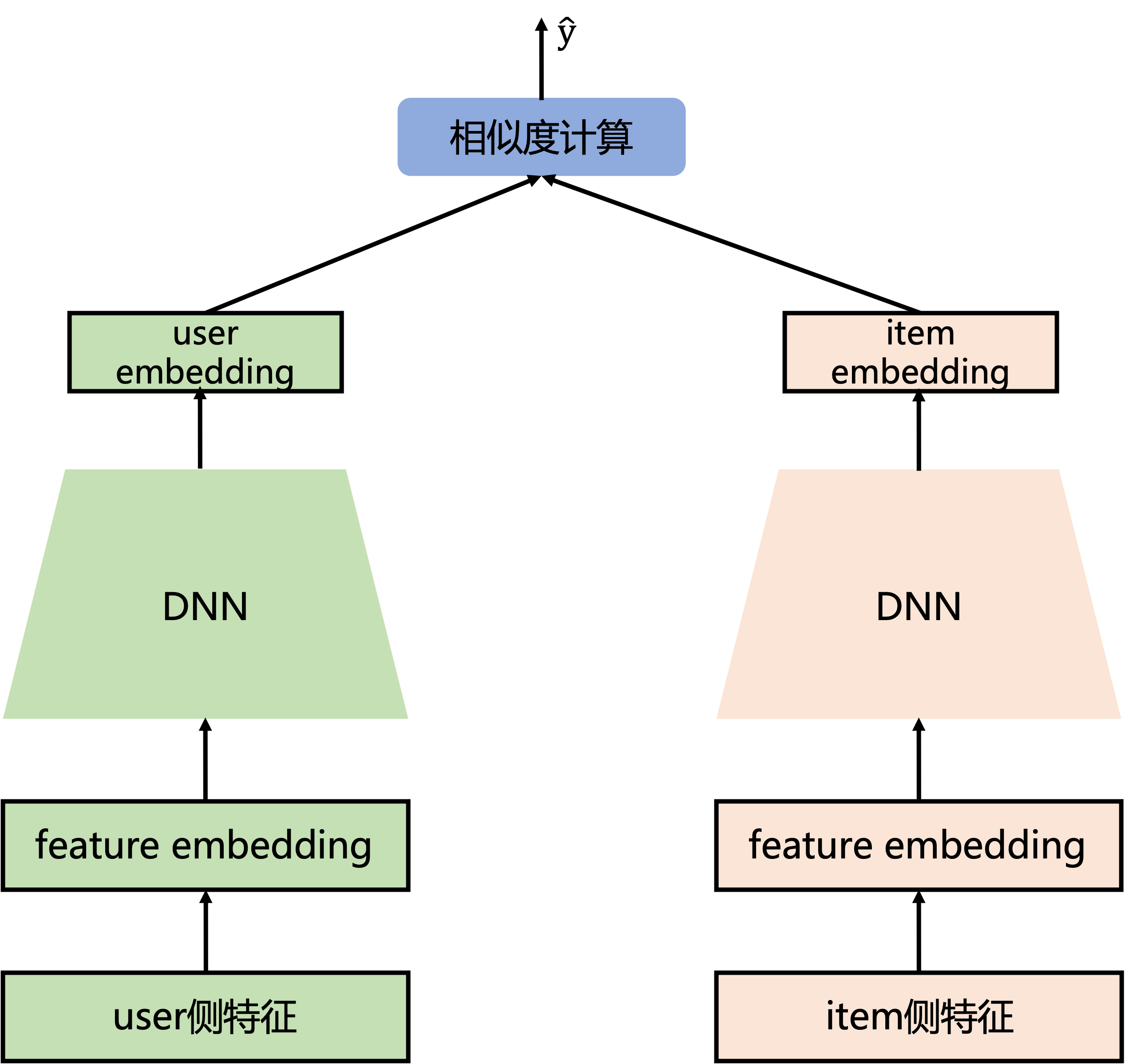
双塔模型结构简单，一个user塔，另一个item塔，两边的DNN机构最后一层（全连接层）隐藏单元个数相同，保证user embedding和item embedding维度相同，后面相似度计算（如cos内积计算），损失函数使用二分类交叉熵损失函数。DSSM模型无法像deepFM一样使用user和item的交叉特征。

业界推荐系统常用多路召回（如CF召回、语义向量召回等，其中DSSM也是语义向量召回的其中一种），DSSM离线训练和普通的DNN训练相同。某baidu大佬有言：精排是特征的艺术，召回是样本的艺术。

• DSSM召回的样本中：
  • 正样本就是曝光给用户并且用户点击的item；
  • 负样本：常见错误是直接使用曝光并且没被user点击的item，但是会导致SSB（sample selection bias）样本选择偏差问题——因为召回在线时时从全量候选item中召回，而不是从有曝光的item中召回。

DSSM原始论文里的做法：只有正样本, 记为 $D^{+}$, 对于用户 $u_1$, 其正样本就是其点击过的 item, 负样本则是随机从 $D^{+}$(不包含 $u_1$ 点击过的item) 中随机选择4个item作为负样本。

2.2 模型原理

三、模型代码

这里我们使用movielen原始的数据集，可以看下对应的字段：

3.1 特征预处理

这里使用两种类别的特征，分别是稀疏特征（SparseFeature）和序列特征（SequenceFeature）。

• 对于稀疏特征，是一个离散的、有限的值（例如用户ID，一般会先进行LabelEncoding操作转化为连续整数值），模型将其输入到Embedding层，输出一个Embedding向量。
• 对于序列特征，每一个样本是一个List[SparseFeature]（一般是观看历史、搜索历史等），对于这种特征，默认对于每一个元素取Embedding后平均，输出一个Embedding向量。此外，除了平均，还有拼接，最值等方式，可以在pooling参数中指定。
• torch rechub框架还支持稠密特征（DenseFeature）（下面没有使用这种特征），即一个连续的特征值（例如概率），这种类型一般需归一化处理。

以上三类特征的定义在torch rechub项目中的torch_rechub/basic/features.py。

3.2 DSSM双塔模型代码

可以结合上面的DSSM结构图（两边都是DNN）

双塔模型结构简单，一个user塔，另一个item塔，两边的DNN机构最后一层（全连接层）隐藏单元个数相同，保证user embedding和item embedding维度相同，后面相似度计算（如cos内积计算），损失函数使用二分类交叉熵损失函数。DSSM模型无法像deepFM一样使用user和item的交叉特征。

import torch
from ...basic.layers import MLP, EmbeddingLayer

class DSSM(torch.nn.Module):
    """Deep Structured Semantic Model

    Args:
        user_features (list[Feature Class]): training by the user tower module.
        item_features (list[Feature Class]): training by the item tower module.
        sim_func (str): similarity function, includes `["cosine", "dot"]`, default to "cosine".
        temperature (float): temperature factor for similarity score, default to 1.0.
        user_params (dict): the params of the User Tower module, keys include:`{"dims":list, "activation":str, "dropout":float, "output_layer":bool`}.
        item_params (dict): the params of the Item Tower module, keys include:`{"dims":list, "activation":str, "dropout":float, "output_layer":bool`}.
    """

    def __init__(self, user_features, item_features, user_params, item_params, sim_func="cosine", temperature=1.0):
        super().__init__()
        self.user_features = user_features
        self.item_features = item_features
        # 计算两个塔结果embedding之间的相似度，也可以使用LSH等方法
        self.sim_func = sim_func
        # 温度系数
        self.temperature = temperature
        # 分别计算user和item的emb维度之和
        self.user_dims = sum([fea.embed_dim for fea in user_features])
        self.item_dims = sum([fea.embed_dim for fea in item_features])
        # 构建embedding层，这里是input为特征列表，output对应特征的字典
        self.embedding = EmbeddingLayer(user_features + item_features)
        self.user_mlp = MLP(self.user_dims, output_layer=False, **user_params)
        self.item_mlp = MLP(self.item_dims, output_layer=False, **item_params)
        self.mode = None

    def forward(self, x):
        # user塔
        user_embedding = self.user_tower(x)
        # item塔
        item_embedding = self.item_tower(x)
        if self.mode == "user":
            return user_embedding
        if self.mode == "item":
            return item_embedding
        
        # 计算相似度：cosine-> similarity
        if self.sim_func == "cosine":
            y = torch.cosine_similarity(user_embedding, item_embedding, dim=1)
        elif self.sim_func == "dot":
            y = torch.mul(user_embedding, item_embedding).sum(dim=1)
        else:
            raise ValueError("similarity function only support %s, but got %s" % (["cosine", "dot"], self.sim_func))
        y = y / self.temperature
        return torch.sigmoid(y)

    def user_tower(self, x):
        if self.mode == "item":
            return None
        input_user = self.embedding(x, self.user_features, squeeze_dim=True)  #[batch_size, num_features*deep_dims]
        user_embedding = self.user_mlp(input_user)  #[batch_size, user_params["dims"][-1]]
        return user_embedding

    def item_tower(self, x):
        if self.mode == "user":
            return None
        input_item = self.embedding(x, self.item_features, squeeze_dim=True)  #[batch_size, num_features*embed_dim]
        item_embedding = self.item_mlp(input_item)  #[batch_size, item_params["dims"][-1]]
        return item_embedding

Reference

[1] torch-rechub项目：https://github.com/datawhalechina/torch-rechub
[2] 【推荐系统】DSSM双塔模型浅析
[3] SysRec2016 | Deep Neural Networks for YouTube Recommendations
[4] torch.CROSSENTROPYLOSS的官方解释：https://pytorch.org/docs/stable/generated/torch.nn.CrossEntropyLoss.html?highlight=crossentropyloss#torch.nn.CrossEntropyLoss
[5] youtubeDNN模型介绍：YouTubeDNN
[6] DSSM模型介绍：DSSM
[7] 推荐- Point wise、pairwise及list wise的比较
[8] pairwise、pointwise 、 listwise算法是什么?怎么理解？主要区别是什么？