目录
0. 前言
开始系统的对PyTorch进行学习了,这里记录一些常用的知识点。应该会写的比较长,所以会分好几P,不断补充。参考资料是PyTorch中文官方教程。
1. 常用基本操作
1.1 创建tensor
PyTorch和Numpy很像,基本数据类型是tensor(张量),可以类比Numpy中的ndarray。很多操作也很类似。
# 创建tensor
empty_tensor = torch.empty((5,4))  # 创建空tensor
one_tensor = torch.ones((5,4))  # 创建全1 tensor
zero_tensor = torch.zeros((5,4))  # 创建全0 tensor
rand_tensor = torch.randn((5,4))  # 创建一个均值为0方差为1呈正态分布的随机数 tensor
x = np.arange(20, dtype=np.uint8).reshape(5,4)
my_tensor = torch.tensor(x)  # 直接创建一个 tensor

print('empty_tensor为:\n{}\n'.format(empty_tensor))
print('one_tensor为:\n{}\n'.format(one_tensor))
print('zero_tensor为:\n{}\n'.format(zero_tensor))
print('rand_tensor为:\n{}\n'.format(rand_tensor))
print('my_tensor为:\n{}\n'.format(my_tensor))
print('默认创建的tensor数据类型为:{}'.format(rand_tensor.dtype))
# 结果

empty_tensor为:
tensor([[0.7318, 0.1863, 0.7587, 0.6429],
        [0.3201, 0.3179, 0.0352, 0.7323],
        [0.0854, 0.5935, 0.1961, 1.5056],
        [0.7802, 1.1091, 0.1342, 0.8146],
        [0.4999, 0.9369, 1.3430, 1.4721]])

one_tensor为:
tensor([[1., 1., 1., 1.],
        [1., 1., 1., 1.],
        [1., 1., 1., 1.],
        [1., 1., 1., 1.],
        [1., 1., 1., 1.]])

zero_tensor为:
tensor([[0., 0., 0., 0.],
        [0., 0., 0., 0.],
        [0., 0., 0., 0.],
        [0., 0., 0., 0.],
        [0., 0., 0., 0.]])

rand_tensor为:
tensor([[ 0.9330,  1.8289,  0.3203,  0.2037],
        [ 1.1852, -0.9822, -0.7285, -0.1997],
        [ 1.2682,  0.4202, -0.6674,  0.5696],
        [-0.4077,  0.0978, -2.0078, -0.8946],
        [-2.1411,  0.1916,  0.7203, -0.4228]])

my_tensor为:
tensor([[ 0,  1,  2,  3],
        [ 4,  5,  6,  7],
        [ 8,  9, 10, 11],
        [12, 13, 14, 15],
        [16, 17, 18, 19]], dtype=torch.uint8)

默认创建的tensor数据类型为:torch.float32
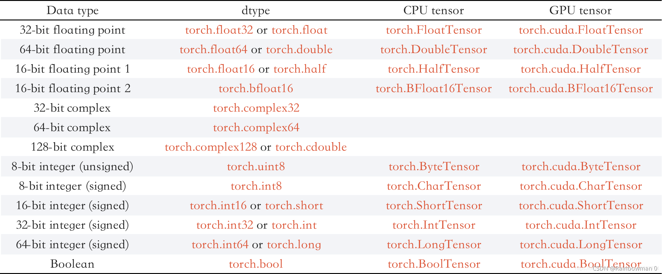
1.2 tensor的基本数据类型:torch.dtype
1.3 改变tensor的基本数据类型:tensor.type()
# 改变tensor的基本数据类型
x = np.arange(20).reshape(5,4)
my_tensor = torch.tensor(x)
print('my_tensor为:\n{}\n'.format(my_tensor))
print('my_tensor的数据类型为:{}\n'.format(my_tensor.dtype))
my_tensor2 = my_tensor.type(torch.float32)
print('my_tensor2为:\n{}\n'.format(my_tensor2))
print('my_tensor2的数据类型为:{}\n'.format(my_tensor2.dtype))
# 结果
my_tensor为:
tensor([[ 0,  1,  2,  3],
        [ 4,  5,  6,  7],
        [ 8,  9, 10, 11],
        [12, 13, 14, 15],
        [16, 17, 18, 19]], dtype=torch.int32)

my_tensor的数据类型为:torch.int32

my_tensor2为:
tensor([[ 0.,  1.,  2.,  3.],
        [ 4.,  5.,  6.,  7.],
        [ 8.,  9., 10., 11.],
        [12., 13., 14., 15.],
        [16., 17., 18., 19.]])

my_tensor2的数据类型为:torch.float32
1.3 改变tensor形状:tensor.view()
x = torch.ones((5,4))
print('x的形状为:{}\n'.format(x.shape))
y = x.view((2,10))
print('y的形状为:{}\n'.format(y.shape))
# 结果
x的形状为:torch.Size([5, 4])

y的形状为:torch.Size([2, 10])
1.4 获得tensor的某个元素的值 : .item()
和ndarray有所区别的是,通过索引的方式无法直接得到一个元素的值:
x = np.arange(20).reshape(5,4)
y = torch.tensor(x)
print('x[0,0]的类型为:\n{}\n'.format(type(x[0,0])))
print('y[0,0]的类型为:\n{}\n'.format(type(y[0,0])))
# 结果
x[0,0]的类型为:
<class 'numpy.int32'>

y[0,0]的类型为:
<class 'torch.Tensor'>
使用item()
x = np.arange(20).reshape(5,4)
y = torch.tensor(x)
print('如果直接访问y[0,0]:', y[0,0])
print('通过item()访问y[0,0]', y[0,0].item())
# 结果
如果直接访问y[0,0]: tensor(0, dtype=torch.int32)
通过item()访问y[0,0] 0
1.5 tensor和ndarray互相转换
1.5.1 tensor —> ndarray: tensor.numpy()
# tensor -> ndarray
x = torch.tensor([1,2,3,4,5])
y = x.numpy()
print('tensor:\n{}\n'.format(x))
print('ndarray:\n{}\n'.format(y))
# 结果
tensor:
tensor([1, 2, 3, 4, 5])

ndarray:
[1 2 3 4 5]
1.5.2 ndarray —> tensor: torch.from_numpy()
# ndarray -> tensor
x = np.array([1,2,3,4,5])
y = torch.from_numpy(x)
print('ndarray:\n{}\n'.format(x))
print('tensor:\n{}\n'.format(y))
# 结果
ndarray:
[1 2 3 4 5]

tensor:
tensor([1, 2, 3, 4, 5], dtype=torch.int32)
2. 自动求微分:tensor.backward()
在PyTorch中,可以用backward()自动求梯度,代码框架如下,注释中有详细讲解:
主要有三点要注意:
(1) 设置tensor的requires_grad属性为True,跟踪tensor后续操作
(2) tensor.backward()自动求梯度
(3) tensor.grad属性记录结果
# 自动求微分
# 设置requires_grad=True才会跟踪tensor的所有操作,之后
# 调用backward()自动计算所有梯度,默认requires_grad=False
x = torch.tensor([1,2], dtype=torch.float64, requires_grad=True)
y = torch.zeros(2, dtype=torch.float64)
y[0] = 2*x[0] + x[1]
y[1] = x[0]**2 + 2*x[1]
out = y.mean()
out.backward()  # 自动求微分
print(x.grad)  # 张量的梯度存储在tensor.grad属性中
# 结果
tensor([2.0000, 1.5000], dtype=torch.float64)
其实很容易理解的:

这里需要说明一点,上面的代码中,我们的out是一个标量(scalar),应用场景挺常见的,比如最终的损失函数(loss)会被定义为一个标量的形式。但如果最后的out是一个张量(tensor)呢(即out是一个向量)?我们来实验一下:
array = np.array([1,2,3,4])
x = torch.tensor(array, dtype=torch.float64, requires_grad=True)
y = torch.zeros(4)
y[0] = 2 * x[0] + x[1]
y[1] = x[0] ** 2 + x[1] ** 2 + x[2]
y[2] = x[2] ** 2 + x[3]
y[3] = x[0] ** 2 + x[2] + x[3] ** 2
y.backward(torch.tensor([1,2,3,4]))
print(x.grad)
# 结果
tensor([14.,  9., 24., 35.], dtype=torch.float64)
此时,我们需要在backward()中传入一个参数 grad_tensor ,形状与tensor.backward()中的tensor形状相同,具体计算过程为:
用grad_tensor×雅各比矩阵,上面代码的具体过程如下图所示:
