Python中的图像处理（第十五章）Python傅里叶变换与霍夫变换（2）

前言

随着人工智能研究的不断兴起，Python的应用也在不断上升，由于Python语言的简洁性、易读性以及可扩展性，特别是在开源工具和深度学习方向中各种神经网络的应用，使得Python已经成为最受欢迎的程序设计语言之一。由于完全开源，加上简单易学、易读、易维护、以及其可移植性、解释性、可扩展性、可扩充性、可嵌入性：丰富的库等等，自己在学习与工作中也时常接触到Python，这个系列文章的话主要就是介绍一些在Python中常用一些例程进行仿真演示！

本系列文章主要参考杨秀章老师分享的代码资源，杨老师博客主页是Eastmount，杨老师兴趣广泛，不愧是令人膜拜的大佬，他过成了我理想中的样子，希望以后有机会可以向他请教学习交流。

因为自己是做图像语音出身的，所以结合《Python中的图像处理》，学习一下Python相关，OpenCV已经在Python上进行了多个版本的维护，所以相比VS，Python的环境配置相对简单，缺什么库直接安装即可。本系列文章例程都是基于Python3.8的环境下进行，所以大家在进行借鉴的时候建议最好在3.8.0版本以上进行仿真。本文继续来对本书第十五章的后6个例程进行介绍。

一. Python准备

如何确定自己安装好了python

win+R输入cmd进入命令行程序

点击“确定”

输入：python，回车

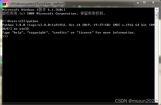
看到Python相关的版本信息，说明Python安装成功。

二. Python仿真

（1）新建一个chapter15_06.py文件，输入以下代码，图片也放在与.py文件同级文件夹下

# -*- coding: utf-8 -*-
import cv2 as cv
import numpy as np
from matplotlib import pyplot as plt
import matplotlib

#读取图像
img = cv.imread('Na.png', 0)

#傅里叶变换
f = np.fft.fft2(img)
fshift = np.fft.fftshift(f)

#设置高通滤波器
rows, cols = img.shape
crow,ccol = int(rows/2), int(cols/2)
fshift[crow-30:crow+30, ccol-30:ccol+30] = 0

#傅里叶逆变换
ishift = np.fft.ifftshift(fshift)
iimg = np.fft.ifft2(ishift)
iimg = np.abs(iimg)

#设置字体
matplotlib.rcParams['font.sans-serif']=['SimHei']

#显示原始图像和高通滤波处理图像
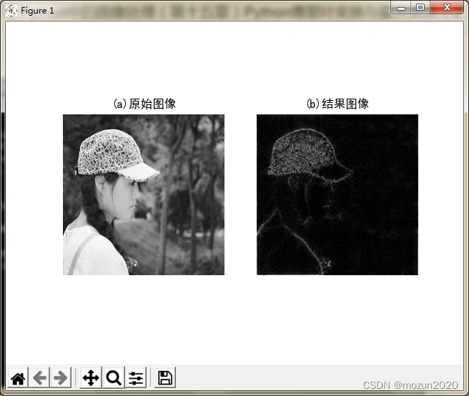
plt.subplot(121), plt.imshow(img, 'gray'), plt.title(u'(a)原始图像')
plt.axis('off')
plt.subplot(122), plt.imshow(iimg, 'gray'), plt.title(u'(b)结果图像')
plt.axis('off')
plt.show()

保存.py文件
输入eixt()退出python，输入命令行进入工程文件目录

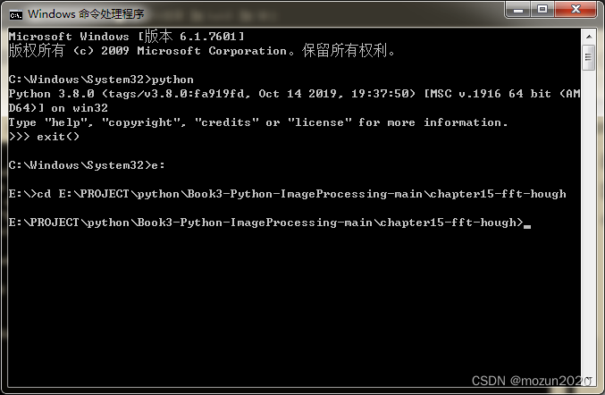
输入以下命令，跑起工程

python chapter15_06.py

没有报错，直接弹出图片，运行成功！

（2）新建一个chapter15_07.py文件，输入以下代码，图片也放在与.py文件同级文件夹下

扫描二维码关注公众号，回复： 14234314 查看本文章

# -*- coding: utf-8 -*-
import cv2
import numpy as np
from matplotlib import pyplot as plt

#读取图像
img = cv2.imread('Na.png', 0)

#傅里叶变换
dft = cv2.dft(np.float32(img), flags = cv2.DFT_COMPLEX_OUTPUT)
fshift = np.fft.fftshift(dft)

#设置低通滤波器
rows, cols = img.shape
crow,ccol = int(rows/2), int(cols/2) #中心位置
mask = np.zeros((rows, cols, 2), np.uint8)
mask[crow-30:crow+30, ccol-30:ccol+30] = 1

#掩膜图像和频谱图像乘积
f = fshift * mask
print(f.shape, fshift.shape, mask.shape)


#傅里叶逆变换
ishift = np.fft.ifftshift(f)
iimg = cv2.idft(ishift)
res = cv2.magnitude(iimg[:,:,0], iimg[:,:,1])

#显示原始图像和低通滤波处理图像
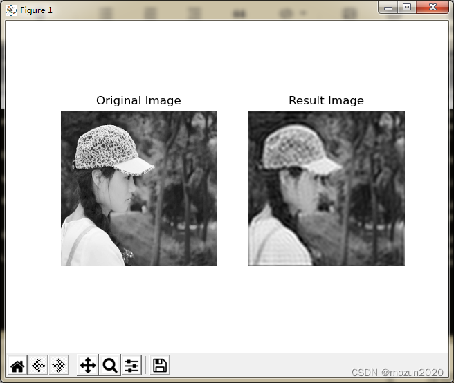
plt.subplot(121), plt.imshow(img, 'gray'), plt.title('Original Image')
plt.axis('off')
plt.subplot(122), plt.imshow(res, 'gray'), plt.title('Result Image')
plt.axis('off')
plt.show()

保存.py文件输入以下命令，跑起工程

python chapter15_07.py

没有报错，直接打印数据，弹出图片，运行成功！

（3）新建一个chapter15_08.py文件，输入以下代码，图片也放在与.py文件同级文件夹下

# -*- coding: utf-8 -*-
import cv2
import numpy as np
from matplotlib import pyplot as plt
import matplotlib

#读取图像
img = cv2.imread('lines.png')

#灰度变换
gray = cv2.cvtColor(img, cv2.COLOR_BGR2GRAY)

#转换为二值图像
edges = cv2.Canny(gray, 50, 150)

#显示原始图像
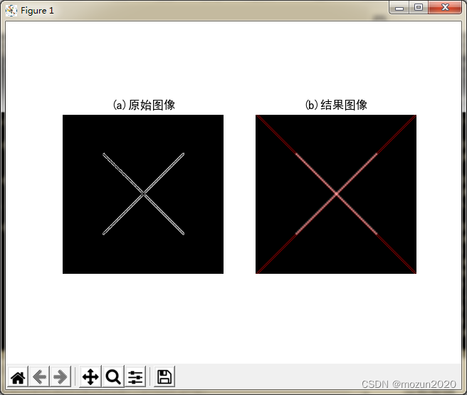
plt.subplot(121), plt.imshow(edges, 'gray'), plt.title(u'(a)原始图像')
plt.axis('off')

#霍夫变换检测直线
lines = cv2.HoughLines(edges, 1, np.pi / 180, 160)

#转换为二维
line = lines[:, 0, :] 

#将检测的线在极坐标中绘制 
for rho,theta in line[:]: 
    a = np.cos(theta)
    b = np.sin(theta)
    x0 = a * rho
    y0 = b * rho
    print(x0, y0)
    x1 = int(x0 + 1000 * (-b))
    y1 = int(y0 + 1000 * (a))
    x2 = int(x0 - 1000 * (-b))
    y2 = int(y0 - 1000 * (a))
    print(x1, y1, x2, y2)
    #绘制直线
    cv2.line(img, (x1, y1), (x2, y2), (255, 0, 0), 1)

#设置字体
matplotlib.rcParams['font.sans-serif']=['SimHei']

#显示处理图像
plt.subplot(122), plt.imshow(img, 'gray'), plt.title(u'(b)结果图像')
plt.axis('off')
plt.show()

保存.py文件输入以下命令，跑起工程

python chapter15_08.py

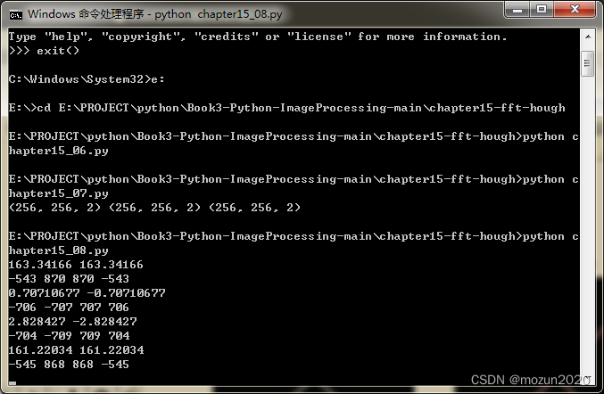
没有报错，直接打印数据，弹出图片，运行成功！

（4）新建一个chapter15_09.py文件，输入以下代码，图片也放在与.py文件同级文件夹下

# -*- coding: utf-8 -*-
import cv2
import numpy as np
from matplotlib import pyplot as plt
import matplotlib

#读取图像
img = cv2.imread('judge.png')

#灰度转换
gray = cv2.cvtColor(img, cv2.COLOR_BGR2GRAY)

#转换为二值图像
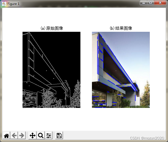
edges = cv2.Canny(gray, 50, 200)

#显示原始图像
plt.subplot(121), plt.imshow(edges, 'gray'), plt.title(u'(a)原始图像')
plt.axis('off')

#霍夫变换检测直线
minLineLength = 60
maxLineGap = 10
lines = cv2.HoughLinesP(edges, 1, np.pi/180, 30, minLineLength, maxLineGap)

#绘制直线
lines1 = lines[:, 0, :]
for x1,y1,x2,y2 in lines1[:]:
    cv2.line(img, (x1,y1), (x2,y2), (255,0,0), 2)

res = cv2.cvtColor(img, cv2.COLOR_BGR2RGB)

#设置字体
matplotlib.rcParams['font.sans-serif']=['SimHei']

#显示处理图像
plt.subplot(122), plt.imshow(res), plt.title(u'(b)结果图像')
plt.axis('off')
plt.show()

保存.py文件输入以下命令，跑起工程

python chapter15_09.py

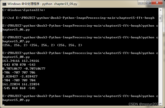
没有报错，直接弹出图片，运行成功！

（5）新建一个chapter15_10.py文件，输入以下代码，图片也放在与.py文件同级文件夹下

# -*- coding: utf-8 -*-
import cv2
import numpy as np
from matplotlib import pyplot as plt

#读取图像
img = cv2.imread('test01.png')

#灰度转换
gray = cv2.cvtColor(img, cv2.COLOR_BGR2GRAY)

#显示原始图像
plt.subplot(121), plt.imshow(gray, 'gray'), plt.title('Input Image')
plt.axis('off')

#霍夫变换检测圆
#circles1 = cv2.HoughCircles(gray, cv2.HOUGH_GRADIENT, 1, 100,
#                           param1=100, param2=30, minRadius=200, maxRadius=300)

circles1 = cv2.HoughCircles(gray, cv2.HOUGH_GRADIENT, 1, 20, param2=30)

print(circles1)

#提取为二维
circles = circles1[0, :, :]

#四舍五入取整
circles = np.uint16(np.around(circles))

#绘制圆
for i in circles[:]: 
    cv2.circle(img, (i[0],i[1]), i[2], (255,0,0), 5) #画圆
    cv2.circle(img, (i[0],i[1]), 2, (255,0,255), 10) #画圆心

#显示处理图像
plt.subplot(122), plt.imshow(img), plt.title('Result Image')
plt.axis('off')
plt.show()

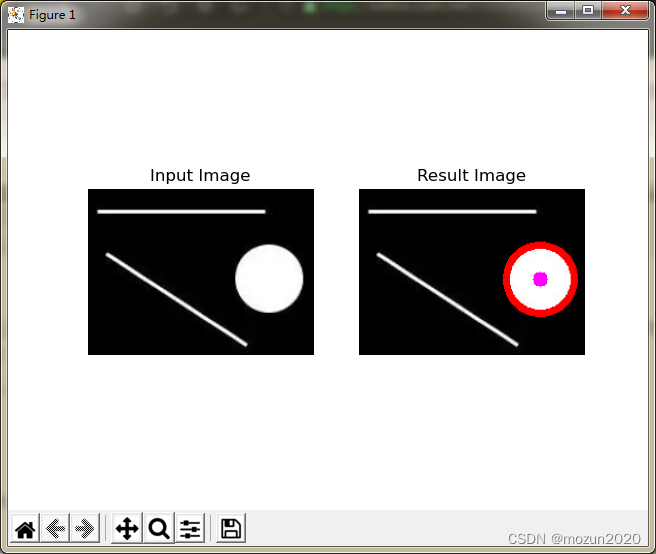
保存.py文件输入以下命令，跑起工程

python chapter15_10.py

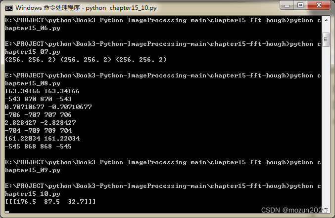
没有报错，直接打印数据，弹出图片，运行成功！

（6）新建一个chapter15_11.py文件，输入以下代码，图片也放在与.py文件同级文件夹下

# -*- coding: utf-8 -*-
import cv2
import numpy as np
from matplotlib import pyplot as plt

#读取图像
img = cv2.imread('eyes.png')

#灰度转换
gray = cv2.cvtColor(img, cv2.COLOR_BGR2GRAY)

#显示原始图像
plt.subplot(121), plt.imshow(gray, 'gray'), plt.title('Input Image')
plt.axis('off')

#霍夫变换检测圆
circles1 = cv2.HoughCircles(gray, cv2.HOUGH_GRADIENT, 1, 20,
                            param1=100, param2=30,
                            minRadius=160, maxRadius=200)
print(circles1)

#提取为二维
circles = circles1[0, :, :]

#四舍五入取整
circles = np.uint16(np.around(circles))

#绘制圆
for i in circles[:]: 
    cv2.circle(img, (i[0],i[1]), i[2], (255,0,0), 5) #画圆
    cv2.circle(img, (i[0],i[1]), 2, (255,0,255), 8) #画圆心

#显示处理图像
plt.subplot(122), plt.imshow(img), plt.title('Result Image')
plt.axis('off')
plt.show()

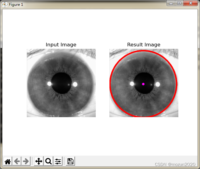
保存.py文件输入以下命令，跑起工程

python chapter15_11.py

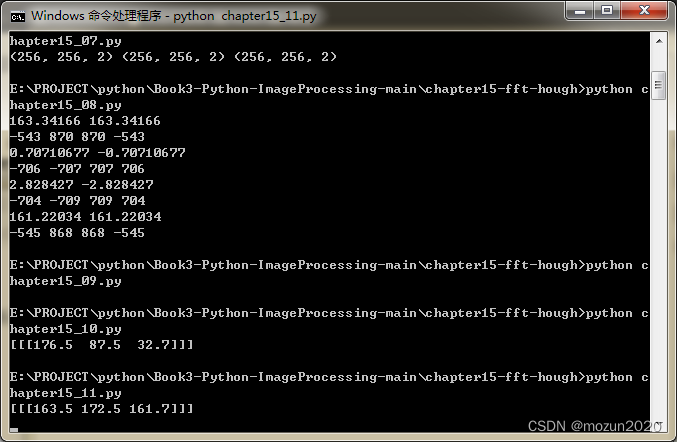
没有报错，直接打印数据，弹出图片，运行成功！

三. 小结

本文主要介绍在Python中调用OpenCV库对图像进行傅里叶变换与傅里叶逆变换，再进行高通滤波，低通滤波处理，以及霍夫变换检测直线与圆等操作。由于本书的介绍比较系统全面，所以会出一个系列文章进行全系列仿真实现，感兴趣的还是建议去原书第十五章深入学习理解。每天学一个Python小知识，大家一起来学习进步阿！

本系列示例主要参考杨老师GitHub源码，安利一下地址：ImageProcessing-Python（喜欢记得给个star哈！）