1、t-SNE概述
t-Distributed Stochastic Neighbor Embedding (t-SNE) 是一种无监督的非线性技术,主要用于数据探索和高维数据的可视化。简单来说,t-SNE 让您对数据在高维空间中的排列方式有一种感觉或直觉。它由 Laurens van der Maatens 和 Geoffrey Hinton 于 2008 年提出。
2、t-SNE 与 PCA
PCA 是在1933年出现的,而t-SNE是在2008年出现的。
PCA 是一种线性降维技术,旨在最大化方差并保持较大的成对距离。换句话说,不同的事物最终会相距甚远。这会导致可视化效果不佳,尤其是在处理非线性流形结构时。将流形结构视为任何几何形状,例如:圆柱体、球体、曲线等。
t-SNE 与 PCA 的不同之处在于仅保留小的成对距离或局部相似性,而 PCA 关注的是保留大的成对距离以最大化方差。Laurens 使用图1 中的 Swiss Roll 数据集很好地说明了 PCA 和 t-SNE 方法。您可以看到,由于这个玩具数据集(流形)的非线性和保留较大的距离,PCA 会错误地保留数据的结构。
使用 t-SNE(实线)与最大化方差 PCA保持小距离

3、t-SNE 的工作原理
t-SNE 算法包括两个主要阶段。首先,t-SNE 在成对的高维对象上构建概率分布,这样相似的对象被赋予更高的概率,而不同的点被赋予更低的概率。其次,t-SNE 定义了低维地图中点的相似概率分布,并且它最小化了两个分布之间关于地图中点位置的Kullback-Leibler 散度(KL散度)。虽然原始算法使用对象之间的欧几里得距离作为其相似性度量的基础,但可以酌情更改。
t-SNE 已在广泛的应用中用于可视化,包括基因组学、计算机安全研究、自然语言处理、音乐分析、癌症研究、生物信息学、地质领域解释、和生物医学信号处理。
4、sklearn中的TSNE
python中的TSNE函数原型如下,详情可访问sklearn。matlab也实现了TSNE。
class sklearn.manifold.TSNE(n_components=2, *, perplexity=30.0, early_exaggeration=12.0, learning_rate=‘warn’, n_iter=1000, n_iter_without_progress=300, min_grad_norm=1e-07, metric=‘euclidean’, init=‘warn’, verbose=0, random_state=None, method=‘barnes_hut’, angle=0.5, n_jobs=None, square_distances=‘legacy’)[source]
其中perplexity是比较敏感的参数,从某种意义上说,该参数是对每个点的近邻数量的猜测。
看下面的示例,最左侧是原始分布,右侧五张图均为迭代5000次,但是perplexity分别为2、5、30、50、100,可以看出perplexity设置不同参数对于可视化影响非常大。

5、 相关示例
参考代码,我们将从在 MNIST 数据集的一部分上执行 t-SNE 开始。MNIST 数据集由从 0 到 9 的手绘数字图像组成。准确分类每个数字是一个hello world级别的机器学习挑战。我们可以使用 sklearn 加载 MNIST 数据集。
from sklearn.datasets import fetch_openml
import numpy as np
import matplotlib.pyplot as plt

# Load the MNIST data
X, y = fetch_openml('mnist_784', version=1, return_X_y=True, as_frame=False)

# Randomly select 1000 samples for performance reasons
np.random.seed(100)
subsample_idc = np.random.choice(X.shape[0], 1000, replace=False)
X = X[subsample_idc,:]
y = y[subsample_idc]

# Show two example images
fig, ax = plt.subplots(1,2)
ax[0].imshow(X[11,:].reshape(28,28), 'Greys')
ax[1].imshow(X[15,:].reshape(28,28), 'Greys')
ax[0].set_title("Label 3")
ax[1].set_title("Label 8")

X.shape
# (1000, 784)
# 1000 Samples with 784 features
y.shape
# (1000,)
# 1000 labels
np.unique(y)
# array(['0', '1', '2', '3', '4', '5', '6', '7', '8', '9'], dtype=object)
# The 10 classes of the images

from sklearn.manifold import TSNE
import pandas as pd
import seaborn as sns

# We want to get TSNE embedding with 2 dimensions
n_components = 2
tsne = TSNE(n_components)
tsne_result = tsne.fit_transform(X)
tsne_result.shape
# (1000, 2)
# Two dimensions for each of our images

# Plot the result of our TSNE with the label color coded
# A lot of the stuff here is about making the plot look pretty and not TSNE
tsne_result_df = pd.DataFrame({

    'tsne_1': tsne_result[:,0], 'tsne_2': tsne_result[:,1], 'label': y})
fig, ax = plt.subplots(1)
sns.scatterplot(x='tsne_1', y='tsne_2', hue='label', data=tsne_result_df, ax=ax,s=120)
lim = (tsne_result.min()-5, tsne_result.max()+5)
ax.set_xlim(lim)
ax.set_ylim(lim)
ax.set_aspect('equal')
ax.legend(bbox_to_anchor=(1.05, 1), loc=2, borderaxespad=0.0)
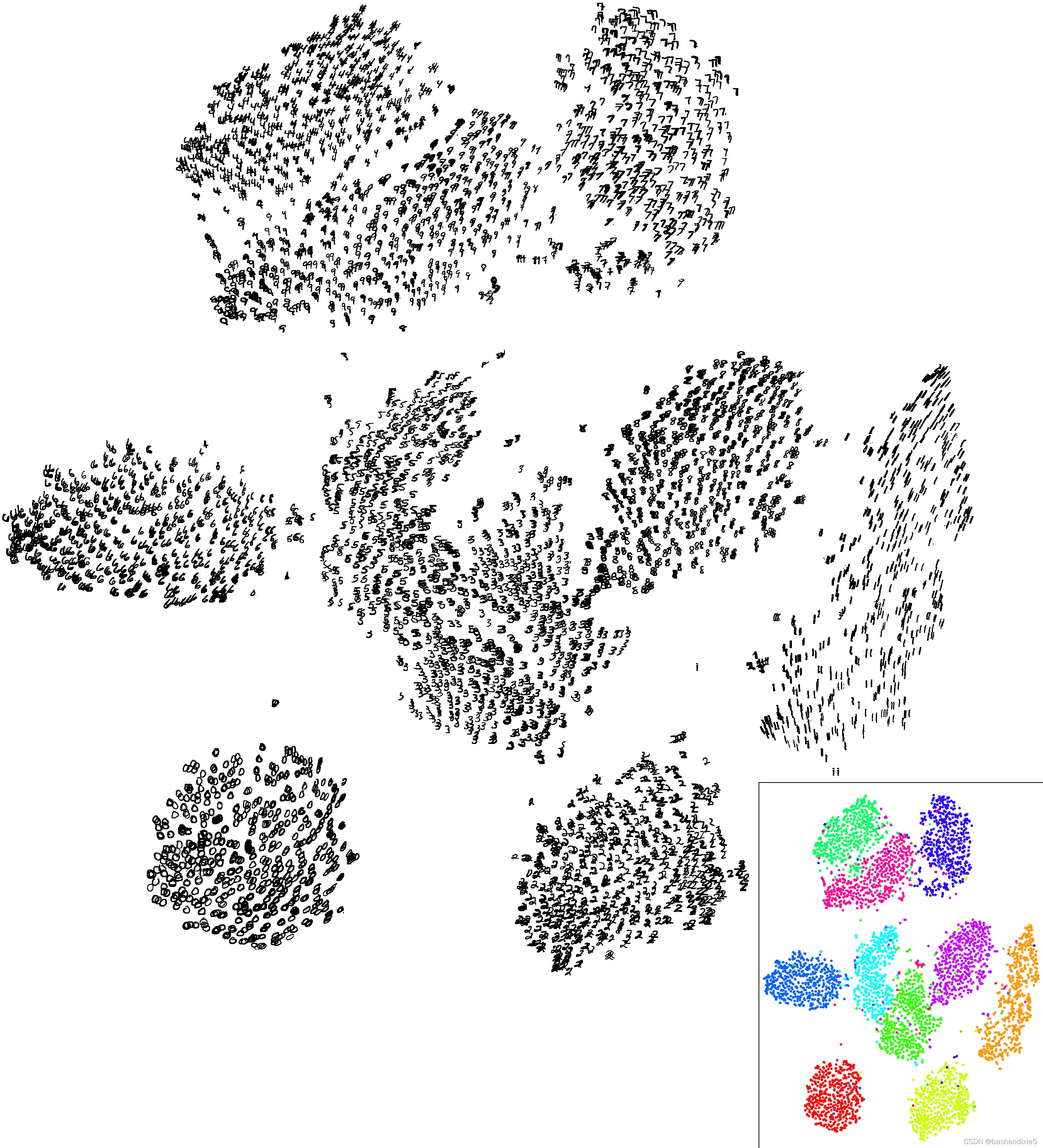
MNIST 子样本上的 t-SNE 示例

MNIST 数据集(二维)上的测试结果
olivetti人脸识别测试结果

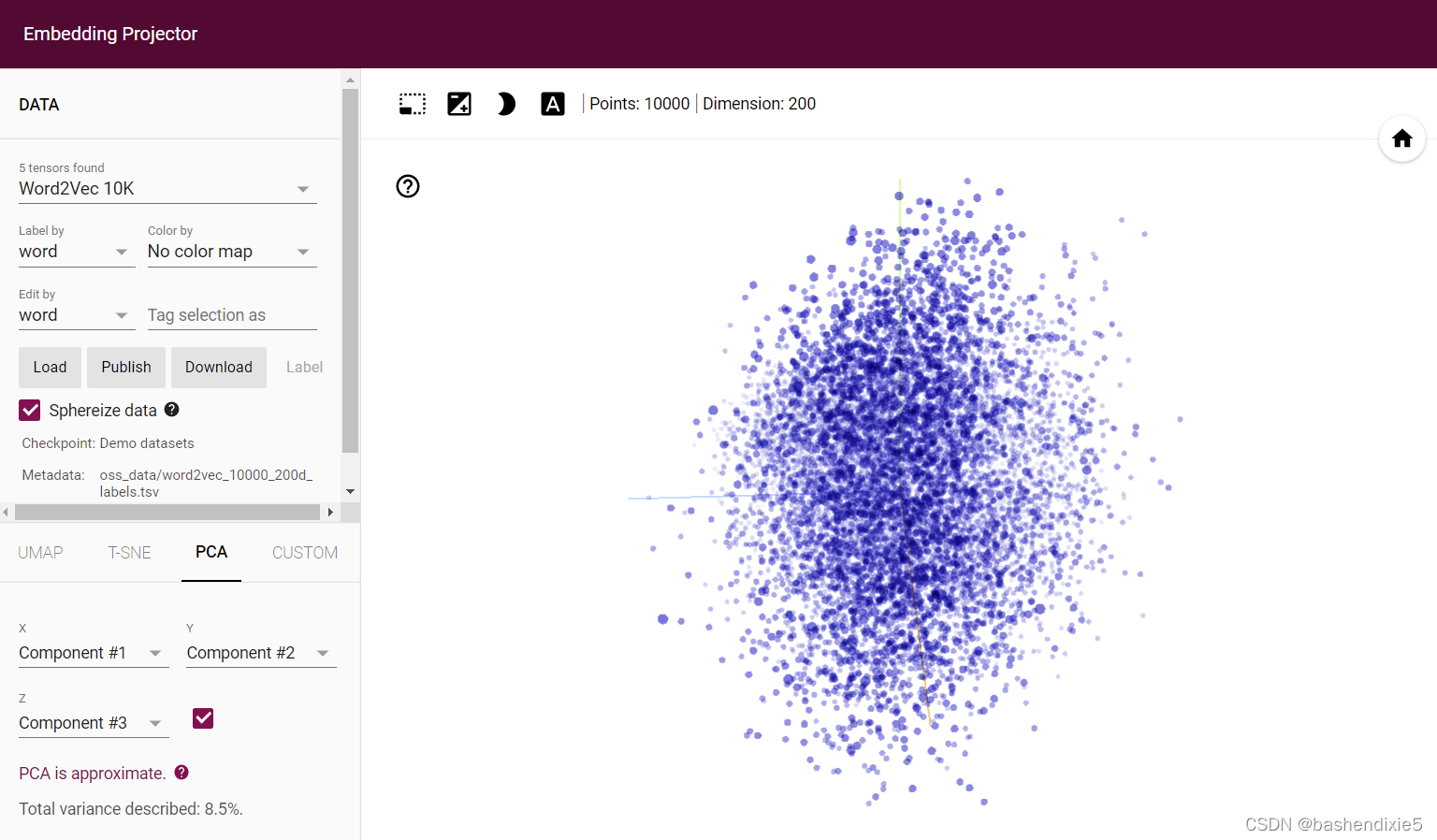
6、tensorflow在线可视化
下面的网址是可视化工具,其中可选一些数据集,以及可选降维方式包括UMAP、TSNE、PCA、自定义等等。
7、其它参考
https://projector.tensorflow.org/
https://lvdmaaten.github.io/tsne/
https://distill.pub/2016/misread-tsne/
https://danielmuellerkomorowska.com/2021/01/05/introduction-to-t-sne-in-python-with-scikit-learn/