数据分析(八)之pandas常用统计方法小练习

pandas常用统计方法

在这里插入图片描述

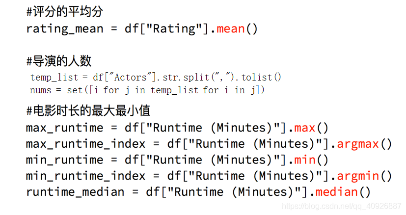
练习1：假设现在我们有一组从2006年到2016年1000部最流行的电影数据，我们想知道这些电影数据中评分的平均分，导演的人数等信息，我们应该怎么获取？
数据来源：https://www.kaggle.com/damianpanek/sunday-eda/data

# coding=utf-8
import pandas as pd
import numpy as np

file_path = "IMDB-Movie-Data.csv"
df = pd.read_csv(file_path)

# print(df.info())

# print(df.head(1))  # 打印一条数据，查看数据都有那些元素

# 获取平均评分
print(df["Rating"].mean())

# 导演的人数
# print(len(set(df["Director"].tolist())))
print(len(df["Director"].unique()))

# 获取演员的人数
temp_actors_list = df["Actors"].str.split(", ").tolist()
actors_list = [i for j in temp_actors_list for i in j]
actors_num = len(set(actors_list))
print(actors_num)

输出：
6.723199999999999
644
2015

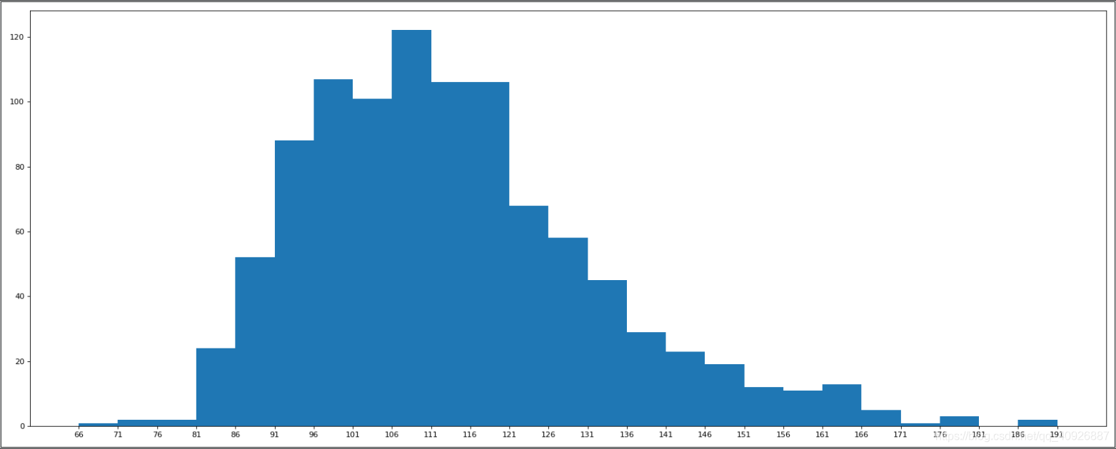
2. 练习2：对于这一组电影数据，如果我们想rating，runtime的分布情况，应该如何呈现数据？
播放时长的分布情况

# coding=utf-8
import pandas as pd
from matplotlib import pyplot as plt

file_path = "./IMDB-Movie-Data.csv"

df = pd.read_csv(file_path)
# print(df.head(1))
# print(df.info())

# rating,runtime分布情况
# 选择图形，直方图
# 准备数据
runtime_data = df["Runtime (Minutes)"].values

max_runtime = runtime_data.max()
min_runtime = runtime_data.min()
print(max_runtime, min_runtime)

# 计算组数
print(max_runtime - min_runtime)
num_bin = (max_runtime - min_runtime) // 5

# 设置图形的大小
plt.figure(figsize=(20, 8), dpi=80)
plt.hist(runtime_data, num_bin)
plt.xticks(range(min_runtime, max_runtime+5, 5))
# _x = [min_runtime]
# i = min_runtime
# while i <= max_runtime + 0.5:
#     i = i + 0.5
#     _x.append(i)
#
# plt.xticks(_x)

plt.show()

输出：
在这里插入图片描述
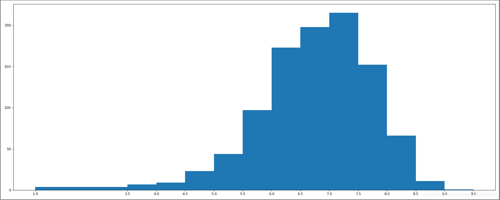
评分的分布情况

import numpy as np
from matplotlib import pyplot as plt

runtime_data = np.array(
    [8.1, 7.0, 7.3, 7.2, 6.2, 6.1, 8.3, 6.4, 7.1, 7.0, 7.5, 7.8, 7.9, 7.7, 6.4, 6.6, 8.2, 6.7, 8.1, 8.0, 6.7, 7.9, 6.7,
     6.5, 5.3, 6.8, 8.3, 4.7, 6.2, 5.9, 6.3, 7.5, 7.1, 8.0, 5.6, 7.9, 8.6, 7.6, 6.9, 7.1, 6.3, 7.5, 2.7, 7.2, 6.3, 6.7,
     7.3, 5.6, 7.1, 3.7, 8.1, 5.8, 5.6, 7.2, 9.0, 7.3, 7.2, 7.4, 7.0, 7.5, 6.7, 6.8, 6.5, 4.1, 8.5, 7.7, 7.4, 8.1, 7.5,
     7.2, 5.9, 7.1, 7.5, 6.8, 8.1, 7.1, 8.1, 8.3, 7.3, 5.3, 8.8, 7.9, 8.2, 8.1, 7.2, 7.0, 6.4, 7.8, 7.8, 7.4, 8.1, 7.0,
     8.1, 7.1, 7.4, 7.4, 8.6, 5.8, 6.3, 8.5, 7.0, 7.0, 8.0, 7.9, 7.3, 7.7, 5.4, 6.3, 5.8, 7.7, 6.3, 8.1, 6.1, 7.7, 8.1,
     5.8, 6.2, 8.8, 7.2, 7.4, 6.7, 6.7, 6.0, 7.4, 8.5, 7.5, 5.7, 6.6, 6.4, 8.0, 7.3, 6.0, 6.4, 8.5, 7.1, 7.3, 8.1, 7.3,
     8.1, 7.1, 8.0, 6.2, 7.8, 8.2, 8.4, 8.1, 7.4, 7.6, 7.6, 6.2, 6.4, 7.2, 5.8, 7.6, 8.1, 4.7, 7.0, 7.4, 7.5, 7.9, 6.0,
     7.0, 8.0, 6.1, 8.0, 5.2, 6.5, 7.3, 7.3, 6.8, 7.9, 7.9, 5.2, 8.0, 7.5, 6.5, 7.6, 7.0, 7.4, 7.3, 6.7, 6.8, 7.0, 5.9,
     8.0, 6.0, 6.3, 6.6, 7.8, 6.3, 7.2, 5.6, 8.1, 5.8, 8.2, 6.9, 6.3, 8.1, 8.1, 6.3, 7.9, 6.5, 7.3, 7.9, 5.7, 7.8, 7.5,
     7.5, 6.8, 6.7, 6.1, 5.3, 7.1, 5.8, 7.0, 5.5, 7.8, 5.7, 6.1, 7.7, 6.7, 7.1, 6.9, 7.8, 7.0, 7.0, 7.1, 6.4, 7.0, 4.8,
     8.2, 5.2, 7.8, 7.4, 6.1, 8.0, 6.8, 3.9, 8.1, 5.9, 7.6, 8.2, 5.8, 6.5, 5.9, 7.6, 7.9, 7.4, 7.1, 8.6, 4.9, 7.3, 7.9,
     6.7, 7.5, 7.8, 5.8, 7.6, 6.4, 7.1, 7.8, 8.0, 6.2, 7.0, 6.0, 4.9, 6.0, 7.5, 6.7, 3.7, 7.8, 7.9, 7.2, 8.0, 6.8, 7.0,
     7.1, 7.7, 7.0, 7.2, 7.3, 7.6, 7.1, 7.0, 6.0, 6.1, 5.8, 5.3, 5.8, 6.1, 7.5, 7.2, 5.7, 7.7, 7.1, 6.6, 5.7, 6.8, 7.1,
     8.1, 7.2, 7.5, 7.0, 5.5, 6.4, 6.7, 6.2, 5.5, 6.0, 6.1, 7.7, 7.8, 6.8, 7.4, 7.5, 7.0, 5.2, 5.3, 6.2, 7.3, 6.5, 6.4,
     7.3, 6.7, 7.7, 6.0, 6.0, 7.4, 7.0, 5.4, 6.9, 7.3, 8.0, 7.4, 8.1, 6.1, 7.8, 5.9, 7.8, 6.5, 6.6, 7.4, 6.4, 6.8, 6.2,
     5.8, 7.7, 7.3, 5.1, 7.7, 7.3, 6.6, 7.1, 6.7, 6.3, 5.5, 7.4, 7.7, 6.6, 7.8, 6.9, 5.7, 7.8, 7.7, 6.3, 8.0, 5.5, 6.9,
     7.0, 5.7, 6.0, 6.8, 6.3, 6.7, 6.9, 5.7, 6.9, 7.6, 7.1, 6.1, 7.6, 7.4, 6.6, 7.6, 7.8, 7.1, 5.6, 6.7, 6.7, 6.6, 6.3,
     5.8, 7.2, 5.0, 5.4, 7.2, 6.8, 5.5, 6.0, 6.1, 6.4, 3.9, 7.1, 7.7, 6.7, 6.7, 7.4, 7.8, 6.6, 6.1, 7.8, 6.5, 7.3, 7.2,
     5.6, 5.4, 6.9, 7.8, 7.7, 7.2, 6.8, 5.7, 5.8, 6.2, 5.9, 7.8, 6.5, 8.1, 5.2, 6.0, 8.4, 4.7, 7.0, 7.4, 6.4, 7.1, 7.1,
     7.6, 6.6, 5.6, 6.3, 7.5, 7.7, 7.4, 6.0, 6.6, 7.1, 7.9, 7.8, 5.9, 7.0, 7.0, 6.8, 6.5, 6.1, 8.3, 6.7, 6.0, 6.4, 7.3,
     7.6, 6.0, 6.6, 7.5, 6.3, 7.5, 6.4, 6.9, 8.0, 6.7, 7.8, 6.4, 5.8, 7.5, 7.7, 7.4, 8.5, 5.7, 8.3, 6.7, 7.2, 6.5, 6.3,
     7.7, 6.3, 7.8, 6.7, 6.7, 6.6, 8.0, 6.5, 6.9, 7.0, 5.3, 6.3, 7.2, 6.8, 7.1, 7.4, 8.3, 6.3, 7.2, 6.5, 7.3, 7.9, 5.7,
     6.5, 7.7, 4.3, 7.8, 7.8, 7.2, 5.0, 7.1, 5.7, 7.1, 6.0, 6.9, 7.9, 6.2, 7.2, 5.3, 4.7, 6.6, 7.0, 3.9, 6.6, 5.4, 6.4,
     6.7, 6.9, 5.4, 7.0, 6.4, 7.2, 6.5, 7.0, 5.7, 7.3, 6.1, 7.2, 7.4, 6.3, 7.1, 5.7, 6.7, 6.8, 6.5, 6.8, 7.9, 5.8, 7.1,
     4.3, 6.3, 7.1, 4.6, 7.1, 6.3, 6.9, 6.6, 6.5, 6.5, 6.8, 7.8, 6.1, 5.8, 6.3, 7.5, 6.1, 6.5, 6.0, 7.1, 7.1, 7.8, 6.8,
     5.8, 6.8, 6.8, 7.6, 6.3, 4.9, 4.2, 5.1, 5.7, 7.6, 5.2, 7.2, 6.0, 7.3, 7.2, 7.8, 6.2, 7.1, 6.4, 6.1, 7.2, 6.6, 6.2,
     7.9, 7.3, 6.7, 6.4, 6.4, 7.2, 5.1, 7.4, 7.2, 6.9, 8.1, 7.0, 6.2, 7.6, 6.7, 7.5, 6.6, 6.3, 4.0, 6.9, 6.3, 7.3, 7.3,
     6.4, 6.6, 5.6, 6.0, 6.3, 6.7, 6.0, 6.1, 6.2, 6.7, 6.6, 7.0, 4.9, 8.4, 7.0, 7.5, 7.3, 5.6, 6.7, 8.0, 8.1, 4.8, 7.5,
     5.5, 8.2, 6.6, 3.2, 5.3, 5.6, 7.4, 6.4, 6.8, 6.7, 6.4, 7.0, 7.9, 5.9, 7.7, 6.7, 7.0, 6.9, 7.7, 6.6, 7.1, 6.6, 5.7,
     6.3, 6.5, 8.0, 6.1, 6.5, 7.6, 5.6, 5.9, 7.2, 6.7, 7.2, 6.5, 7.2, 6.7, 7.5, 6.5, 5.9, 7.7, 8.0, 7.6, 6.1, 8.3, 7.1,
     5.4, 7.8, 6.5, 5.5, 7.9, 8.1, 6.1, 7.3, 7.2, 5.5, 6.5, 7.0, 7.1, 6.6, 6.5, 5.8, 7.1, 6.5, 7.4, 6.2, 6.0, 7.6, 7.3,
     8.2, 5.8, 6.5, 6.6, 6.2, 5.8, 6.4, 6.7, 7.1, 6.0, 5.1, 6.2, 6.2, 6.6, 7.6, 6.8, 6.7, 6.3, 7.0, 6.9, 6.6, 7.7, 7.5,
     5.6, 7.1, 5.7, 5.2, 5.4, 6.6, 8.2, 7.6, 6.2, 6.1, 4.6, 5.7, 6.1, 5.9, 7.2, 6.5, 7.9, 6.3, 5.0, 7.3, 5.2, 6.6, 5.2,
     7.8, 7.5, 7.3, 7.3, 6.6, 5.7, 8.2, 6.7, 6.2, 6.3, 5.7, 6.6, 4.5, 8.1, 5.6, 7.3, 6.2, 5.1, 4.7, 4.8, 7.2, 6.9, 6.5,
     7.3, 6.5, 6.9, 7.8, 6.8, 4.6, 6.7, 6.4, 6.0, 6.3, 6.6, 7.8, 6.6, 6.2, 7.3, 7.4, 6.5, 7.0, 4.3, 7.2, 6.2, 6.2, 6.8,
     6.0, 6.6, 7.1, 6.8, 5.2, 6.7, 6.2, 7.0, 6.3, 7.8, 7.6, 5.4, 7.6, 5.4, 4.6, 6.9, 6.8, 5.8, 7.0, 5.8, 5.3, 4.6, 5.3,
     7.6, 1.9, 7.2, 6.4, 7.4, 5.7, 6.4, 6.3, 7.5, 5.5, 4.2, 7.8, 6.3, 6.4, 7.1, 7.1, 6.8, 7.3, 6.7, 7.8, 6.3, 7.5, 6.8,
     7.4, 6.8, 7.1, 7.6, 5.9, 6.6, 7.5, 6.4, 7.8, 7.2, 8.4, 6.2, 7.1, 6.3, 6.5, 6.9, 6.9, 6.6, 6.9, 7.7, 2.7, 5.4, 7.0,
     6.6, 7.0, 6.9, 7.3, 5.8, 5.8, 6.9, 7.5, 6.3, 6.9, 6.1, 7.5, 6.8, 6.5, 5.5, 7.7, 3.5, 6.2, 7.1, 5.5, 7.1, 7.1, 7.1,
     7.9, 6.5, 5.5, 6.5, 5.6, 6.8, 7.9, 6.2, 6.2, 6.7, 6.9, 6.5, 6.6, 6.4, 4.7, 7.2, 7.2, 6.7, 7.5, 6.6, 6.7, 7.5, 6.1,
     6.4, 6.3, 6.4, 6.8, 6.1, 4.9, 7.3, 5.9, 6.1, 7.1, 5.9, 6.8, 5.4, 6.3, 6.2, 6.6, 4.4, 6.8, 7.3, 7.4, 6.1, 4.9, 5.8,
     6.1, 6.4, 6.9, 7.2, 5.6, 4.9, 6.1, 7.8, 7.3, 4.3, 7.2, 6.4, 6.2, 5.2, 7.7, 6.2, 7.8, 7.0, 5.9, 6.7, 6.3, 6.9, 7.0,
     6.7, 7.3, 3.5, 6.5, 4.8, 6.9, 5.9, 6.2, 7.4, 6.0, 6.2, 5.0, 7.0, 7.6, 7.0, 5.3, 7.4, 6.5, 6.8, 5.6, 5.9, 6.3, 7.1,
     7.5, 6.6, 8.5, 6.3, 5.9, 6.7, 6.2, 5.5, 6.2, 5.6, 5.3])
max_runtime = runtime_data.max()
min_runtime = runtime_data.min()
print(min_runtime, max_runtime)

# 设置不等宽的组距，hist方法中取到的会是一个左闭右开的去见[1.9,3.5)
num_bin_list = [1.9, 3.5]
i = 3.5
while i <= max_runtime:
    i += 0.5
    num_bin_list.append(i)
print(num_bin_list)

# 设置图形的大小
plt.figure(figsize=(20, 8), dpi=80)
# num_bin = (max_runtime - min_runtime) // 0.5 # TypeError: `bins` must be an integer, a string, or an array
plt.hist(runtime_data, num_bin_list)

# xticks让之前的组距能够对应上
plt.xticks(num_bin_list)

plt.show()

输出：
在这里插入图片描述
练习3：字符串离散化案例
对于这一组电影数据，如果我们希望统计电影分类(genre)的情况，应该如何处理数据？

思路：很重要
- 重新构造一个全为0的数组，列名为分类，如果某一条数据中分类出现过，就让0变为1

在这里插入图片描述

准备工作：先查看一下电影有多少种种类

import pandas as pd

file_path = "./IMDB-Movie-Data.csv"

df = pd.read_csv(file_path)
print(df["Genre"])

输出：
0       Action,Adventure,Sci-Fi
1      Adventure,Mystery,Sci-Fi
2               Horror,Thriller
3       Animation,Comedy,Family
4      Action,Adventure,Fantasy
                 ...           
995         Crime,Drama,Mystery
996                      Horror
997         Drama,Music,Romance
998            Adventure,Comedy
999       Comedy,Family,Fantasy
Name: Genre, Length: 1000, dtype: object

开始练习：

# coding=utf-8
import pandas as pd
from matplotlib import pyplot as plt
import numpy as np

file_path = "./IMDB-Movie-Data.csv"

df = pd.read_csv(file_path)
print(df["Genre"].head(3))
# 统计分类的列表
temp_list = df["Genre"].str.split(",").tolist()  # [[],[],[]]

genre_list = list(set([i for j in temp_list for i in j]))

# 构造全为0的数组
zeros_df = pd.DataFrame(np.zeros((df.shape[0], len(genre_list))), columns=genre_list)
# print(zeros_df)

# 给每个电影出现分类的位置赋值1
for i in range(df.shape[0]):
    # zeros_df.loc[0,["Sci-fi","Mucical"]] = 1
    zeros_df.loc[i, temp_list[i]] = 1

# print(zeros_df.head(3))

# 统计每个分类的电影的数量和
genre_count = zeros_df.sum(axis=0)
print(genre_count)

# 排序
genre_count = genre_count.sort_values()
_x = genre_count.index
_y = genre_count.values
# 画图
plt.figure(figsize=(20, 8), dpi=80)
plt.bar(range(len(_x)), _y, width=0.4, color="orange")
plt.xticks(range(len(_x)), _x)
plt.show()

输出的结果：
0     Action,Adventure,Sci-Fi
1    Adventure,Mystery,Sci-Fi
2             Horror,Thriller
Name: Genre, dtype: object

Fantasy      101.0
Music         16.0
Crime        150.0
Romance      141.0
Animation     49.0
Mystery      106.0
War           13.0
Adventure    259.0
Sport         18.0
Comedy       279.0
Thriller     195.0
Action       303.0
Western        7.0
Drama        513.0
Sci-Fi       120.0
Family        51.0
Biography     81.0
Musical        5.0
History       29.0
Horror       119.0
dtype: float64

在这里插入图片描述

第四天学习小结【思维导图】

在这里插入图片描述

数据分析(八)之pandas常用统计方法小练习

pandas常用统计方法

第四天学习小结【思维导图】

猜你喜欢