Categoricals是pandas的一种数据类型,对应于统计学中的Categorical variables(分类变量),分类变量是有限且固定的可能值,例如:gender(性别)、血型、国籍等,与统计学的Categorical variables相比,Categorical类型的数据可以具有特定的顺序,例如:按程度来设定:‘强烈同意’与‘同意’,‘首次观察’与‘二次观察’,但是不能按数值来进行排序操作。
Categorical data的值要么是预设好的类型中的某一个,要么是空值(np.nan)。顺序是由Categories来决定的,而不是按照Categories中各个元素的字母顺序排序的。categories 实例的内部是由类型名字集合和一个整数组成的数组构成的,后者标明了类型集合真正的值。
类别数据型适用于以下场景:
- 仅由几个不同值组成的字符串变量。将这样的字符串变量转换成分类变量将节省一些内存;
- 变量的词汇顺序不同于逻辑顺序。通过转换为类别并指定类别的顺序,排序和最小/最大值将使用逻辑顺序替代词汇顺序;
- 作为对其他python库的一个信号,这个列应该被视为一个分类变量。
一、category的创建及其性质
1.分类变量的创建
(a)用Series创建
pd.Series(["a", "b", "c", "a"], dtype="category")
(b)用dataframe创建
temp_df = pd.DataFrame({'A':pd.Series(["a", "b", "c", "a"], dtype="category"),'B':list('abcd')})
temp_df.dtypes
(c)用内置Categorical类型创建
cat = pd.Categorical(["a", "b", "c", "a"], categories=['a','b','c'])
pd.Series(cat)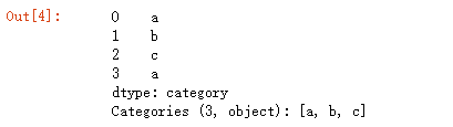
(d)用cut函数创建
默认使用区间类型为标签
pd.cut(np.random.randint(0,60,5), [0,10,30,60])![]()
可指定字符为标签
pd.cut(np.random.randint(0,60,5), [0,10,30,60], right=False, labels=['0-10','10-30','30-60'])![]()
2.分类变量的结构
一个分类变量包括三个部分,元素值(values)、分类类别(categories)、是否有序(order),使用cut函数创建的分类变量默认为有序分类变量。
(a)describe方法
描述了一个分类序列的情况,包括非缺失值个数,元素值类别数(不是分类类别数)、最多出现的元素及其频数
s = pd.Series(pd.Categorical(["a", "b", "c", "a",np.nan], categories=['a','b','c','d']))
s.describe()
(b)categories和ordered属性
查看分类类别和是否排序
#查看分类类别
print(s.cat.categories)
#查看是否排序
print(s.cat.ordered)
3.类别的修改
(a)利用set_categories修改
修改分类,但本身值不会变化
s = pd.Series(pd.Categorical(["a", "b", "c", "a",np.nan], categories=['a','b','c','d']))
s.cat.set_categories(['new_a','c'])

(b)利用rename_categories修改
该方法是会把值和分类同时修改
s = pd.Series(pd.Categorical(["a", "b", "c", "a",np.nan], categories=['a','b','c','d']))
s.cat.rename_categories(['new_%s'%i for i in s.cat.categories])
利用字典修改值
s.cat.rename_categories({'a':'new_a','b':'new_b'})
(c)利用add_categories添加
s = pd.Series(pd.Categorical(["a", "b", "c", "a",np.nan], categories=['a','b','c','d']))
s.cat.add_categories(['e'])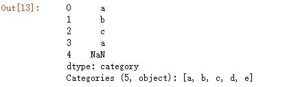
(d)利用remove_categories移除
s = pd.Series(pd.Categorical(["a", "b", "c", "a",np.nan], categories=['a','b','c','d']))
s.cat.remove_categories(['d'])
(e)删除元素值未出现的分类类型
s = pd.Series(pd.Categorical(["a", "b", "c", "a",np.nan], categories=['a','b','c','d']))
s.cat.remove_unused_categories()
二、分类变量的排序
分类数据类型分为有序和无序,
1.序的建立
(a)一般来说会将一个序列转为有序变量,可以利用as_ordered方法
s = pd.Series(["a", "d", "c", "a"]).astype('category').cat.as_ordered()
退化为无序变量,只需使用as_unordered
s.cat.as_unordered()(b)利用set_categories方法中的order参数
pd.Series(["a","d","c","a"]).astype('category').cat.set_categories(['a','c','d'],ordered=True)

(c)利用reorder_categories方法
特点在于:新设置的分类必须与原分类为统一集合
s = pd.Series(["a", "d", "c", "a"]).astype('category')
s.cat.reorder_categories(['a','c','d'],ordered=True)
#s.cat.reorder_categories(['a','c'],ordered=True) #报错
#s.cat.reorder_categories(['a','c','d','e'],ordered=True) #报错
2.排序
(a)值排序
s=pd.Series(np.random.choice(['perfect','good','fair','bad','awful'],50)).astype('category')
s.cat.set_categories(['perfect','good','fair','bad','awful'][::-1],ordered=True).head()
s.sort_values(ascending=False).head()
(b)索引排序
df_sort = pd.DataFrame({'cat':s.values,'value':np.random.randn(50)}).set_index('cat')
df_sort.sort_index().head()
三、分类变量的比较操作
1.与标量或等长序列的比较
(a)标量比较
s = pd.Series(["a", "d", "c", "a"]).astype('category')
s == 'a'
(b)等长序列比较
s == list('abcd')
2.与另一分类变量的比较
(a)等式判别(包含等号和不等号)
两个分类变量的等式判别需要满足分类完全相同
s = pd.Series(["a", "d", "c", "a"]).astype('category')
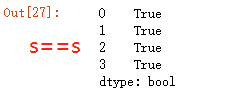
#等号
s == s
#不等于
s != s
#s == s_new #报错
s_new = s.cat.set_categories(['a','d','e'])

(b)不等式判别(包含>=,<=,<,>)
两个分类变量的不等式判别需要满足两个条件:① 分类完全相同 ② 排序完全相同
s = pd.Series(["a", "d", "c", "a"]).astype('category')
#s >= s #报错

s=pd.Series(["a","d","c","a"]).astype('category').cat.reorder_categories(['a','c','d'],ordered=True)
s >= s
练习1:
(a)现在将深度分为七个等级:[0,5,10,15,20,30,50,np.inf],请以深度等级Ⅰ,Ⅱ,Ⅲ,Ⅳ,Ⅴ,Ⅵ,Ⅶ为索引并按照由浅到深的顺序进行排序。
df['new_深度'] = pd.cut(df['深度'],[0,5,10,15,20,30,50,np.inf],labels=['Ⅰ','Ⅱ','Ⅲ','Ⅳ','Ⅴ','Ⅵ','Ⅶ'])
df.set_index('new_深度').sort_index().head()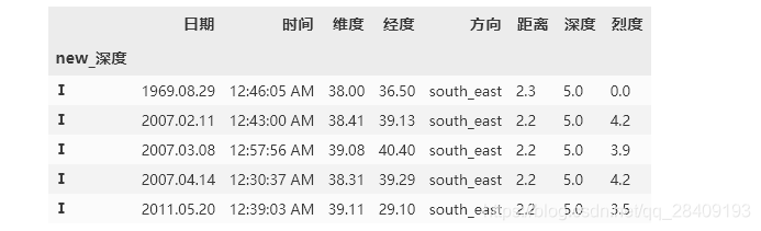
(b)在(a)的基础上,将烈度分为4个等级:[0,3,4,5,np.inf],依次对南部地区的深度和烈度等级建立多级索引排序。
df['new_深度'] = pd.cut(df['深度'],[0,5,10,15,20,30,50,np.inf],labels=['Ⅰ','Ⅱ','Ⅲ','Ⅳ','Ⅴ','Ⅵ','Ⅶ'])
df['new_烈度'] = pd.cut(df['烈度'],[0,3,4,5,np.inf],labels=['Ⅰ','Ⅱ','Ⅲ','Ⅳ'])
df.set_index(['new_深度','new_烈度']).sort_index().head()
可以看到按烈度排序的话,直接从Ⅱ开始的,所以,更改一下数据范围:
df['new_深度'] = pd.cut(df['深度'],[0,5,10,15,20,30,50,np.inf],labels=['Ⅰ','Ⅱ','Ⅲ','Ⅳ','Ⅴ','Ⅵ','Ⅶ'])
df['new_烈度'] = pd.cut(df['烈度'],[-1e-10,3,4,5,np.inf],labels=['Ⅰ','Ⅱ','Ⅲ','Ⅳ'])
df.set_index(['new_深度','new_烈度']).sort_index().head()