The quality of the data and the amount of useful information that it contains are key factors that determine how well a machine learning algorithm can learn. Therefore, it is absolutely critical that we make sure to examine and preprocess a dataset before we feed it to a learning algorithm. In this chapter, we will discuss the essential data preprocessing techniques that will help us build good machine learning models.
The topics that we will cover in this chapter are as follows:

Removing and imputing插补 missing values from the dataset
Getting categorical data into shape for machine learning algorithms
Selecting relevant features for the model construction

Dealing with missing data

It is not uncommon in real-world applications for our samples to be missing one or more values for various reasons. There could have been an error in the data collection process, certain measurements are not applicable, or particular fields could
have been simply left blank in a survey, for example. We typically see missing values as the blank spaces in our data table or as placeholder strings such as NaN, which stands for not a number, or NULL (a commonly used indicator of unknown values in relational databases).

Unfortunately, most computational tools are unable to handle such missing values, or produce unpredictable results if we simply ignore them. Therefore, it is crucial that we take care of those missing values before we proceed with further analyses. In this section, we will work through several practical techniques for dealing with missing values by removing entries from our dataset or imputing missing values from other samples and features.

Identifying missing values in tabular data

But before we discuss several techniques for dealing with missing values, let's create a simple example data frame from a Comma-separated Values (CSV) file to get a better grasp of the problem:

# CSV-formatted data
csv_data = \
'''A,B,C,D
1.0,2.0,3.0,4.0
5.0,6.0,,8.0
10.0,11.0,12.0,'''
# CSV-formatted data

# If you are using Python 2.7, you need
# to convert the string to unicode:

if (sys.version_info < (3, 0)):
    csv_data = unicode(csv_data)

df = pd.read_csv(StringIO(csv_data))
df

Using the preceding code, we read CSV-formatted data into a pandas DataFrame via the read_csv function and noticed that the two missing cells were replaced by NaN. The StringIO function in the preceding code example was simply used for the purposes of illustration. It allows us to read the string assigned to csv_data into a pandas DataFrame as if it was a regular CSV file on our hard drive.

For a larger DataFrame, it can be tedious to look for missing values manually; in this case, we can use the isnull method to return a DataFrame with Boolean values that indicate whether a cell contains a numeric value (False) or if data is missing (True). Using the sum method, we can then return the number of missing values per column as follows:

df.isnull().sum(axis=0)

This way, we can count the number of missing values per column; in the following subsections, we will take a look at different strategies for how to deal with this missing data.

##############################################
Note

Although scikit-learn was developed for working with NumPy arrays, it can sometimes be more convenient to preprocess data using pandas' DataFrame. We can always access the underlying NumPy array of a DataFrame via the values attribute
before we feed it into a scikit-learn estimator:

df.values

##############################################

Eliminating samples or features with missing values

One of the easiest ways to deal with missing data is to simply remove the corresponding features (columns) or samples (rows) from the dataset entirely; rows with missing values can be easily dropped via the dropna method:

df.dropna(axis=0)

Similarly, we can drop columns that have at least one NaN in any row by setting the axis argument to 1:

df.dropna(axis=1)

The dropna method supports several additional parameters that can come in handy:
# only drop rows where all columns are NaN(default axis=0)
# (returns the whole array here since we don't have a row with where all values are NaN

df.dropna(how="all", axis=0)

# drop rows that have less than 4 real values

df.dropna(thresh=4)

# only drop rows where NaN appear in specific columns (here: 'C')

df.dropna(subset=['C'])

Although the removal of missing data seems to be a convenient approach, it also comes with certain disadvantages; for example, we may end up removing too many samples, which will make a reliable analysis impossible. Or, if we remove too many feature columns, we will run the risk of losing valuable information that our classifier needs to discriminate between classes. In the next section, we will thus look at one of the most commonly used alternatives for dealing with missing values: interpolation techniques.

Imputing missing values

Often, the removal of samples or dropping of entire feature columns is simply not feasible, because we might lose too much valuable data. In this case, we can use different interpolation techniques to estimate the missing values from the other training samples in our dataset. One of the most common interpolation techniques is mean imputation, where we simply replace the missing value with the mean value of the entire feature column. A convenient way to achieve this is by using the Imputer class from scikit-learn, as shown in the following code:

# again: our original array
df.values

# impute missing values via the column mean

from sklearn.impute import SimpleImputer
import numpy as np

imr = SimpleImputer(missing_values=np.nan, strategy="mean")
imr = imr.fit(df.values)
imputed_data = imr.transform(df.values)
imputed_data

# 3+12=15/2=7.5 # 4+8=12/2=6

Here, we replaced each NaN value with the corresponding mean, which is separately calculated for each feature column. If we changed the axis=0 setting to axis=1 (sklearn.preprocessing.Imputer(missing_values='NaN', strategy='mean', axis=0, verbose=0, copy=True)[sklearn version 0.17]), we'd calculate the row means.

d=df.values.copy()
np.transpose(d)

# impute missing values via the column mean

from sklearn.impute import SimpleImputer
import numpy as np

imr = SimpleImputer(missing_values=np.nan, strategy="mean")
imr = imr.fit(np.transpose(df.values))
imputed_data = imr.transform(np.transpose(df.values))
imputed_data

#(5+6+8)/3=6.33333333 #(10+11+12)/3=11

Other options for the strategy parameter are median or most_frequent, where the latter replaces the missing values with the most frequent values. This is useful for imputing categorical feature values, for example, a feature column that stores an encoding of color names, such as red, green, and blue, and we will encounter examples of such data later in this chapter.

Understanding the scikit-learn estimator API

In the previous section, we used the Imputer class from scikit-learn to impute missing values in our dataset. The Imputer class belongs to the so-called transformer classes in scikit-learn, which are used for data transformation. The two essential methods of those estimators are fit and transform. The fit method is used to learn the parameters from the training data, and the transform method uses those parameters to transform the data. Any data array that is to be transformed needs to have the same number of features as the data array that was used to fit the model. The following figure illustrates how a transformer, fitted on the training data, is used to transform a training dataset as well as a new test dataset:

The classifiers that we used in cp3 A Tour of ML Classifiers_stratify_bincount_likelihood_logistic regression_odds ratio_decay_L2 https://blog.csdn.net/Linli522362242/article/details/96480059, belong to the so-called estimators in scikit-learn with an API that is conceptually very similar to the transformer class. Estimators have a predict method but can also have a transform method, as we will see later in this chapter. As you may recall, we also used the fit method to learn the parameters of a model when we trained those estimators for classification. However, in supervised learning tasks, we additionally provide the class labels for fitting the model, which can then be used to make predictions about new data samples via the predict method, as illustrated in the following figure:

Handling categorical data

So far, we have only been working with numerical values. However, it is not uncommon that real-world datasets contain one or more categorical feature columns. In this section, we will make use of simple yet effective examples to see how we deal with this type of data in numerical computing libraries.

Nominal and ordinal features

When we are talking about categorical data, we have to further distinguish between nominal and ordinal features. Ordinal features can be understood as categorical values that can be sorted or ordered. For example, t-shirt size would be an ordinal feature, because we can define an order XL > L > M. In contrast, nominal features don't imply any order and, to continue with the previous example, we could think of t-shirt color as a nominal feature since it typically doesn't make sense to say that, for example, red is larger than blue.

Creating an example dataset

Before we explore different techniques to handle such categorical data, let's create a new DataFrame to illustrate the problem:

import pandas as pd

df = pd.DataFrame([['green', 'M', 10.1, 'clas2'],
                   ['red', 'L', 13.5, 'class1'],
                   ['blue', 'XL', 15.3, 'class2']
                  ])
df.columns = ['color', 'size', 'price', 'classlabel']
df

As we can see in the preceding output, the newly created DataFrame contains a nominal feature (color), an ordinal feature (size), and a numerical feature (price) column. The class labels (assuming that we created a dataset for a supervised learning task) are stored in the last column. The learning algorithms for classification that we discuss in this book do not use ordinal information in class labels.

Mapping ordinal features

To make sure that the learning algorithm interprets the ordinal features correctly, we need to convert the categorical string values into integers. Unfortunately, there is no convenient function that can automatically derive the correct order of the labels of our size feature, so we have to define the mapping manually. In the following simple example, let's assume that we know the numerical difference between features, for example, :

size_mapping = {'XL': 3,
                'L': 2,
                'M': 1}
df['size'] = df['size'].map(size_mapping)
df

If we want to transform the integer values back to the original string representation at a later stage, we can simply define a reverse-mapping dictionary inv_size_mapping = {v: k for k, v in size_mapping.items()} that can then be used via the pandas map method on the transformed feature column, similar to the size_mapping dictionary that we used previously. We can use it as follows:

inv_size_mapping = {v: k for k,v in size_mapping.items()} # return a value(k)
df['size'].map(inv_size_mapping)

Encoding class labels

Many machine learning libraries require that class labels are encoded as integer values. Although most estimators for classification in scikit-learn convert class labels to integers internally, it is considered good practice to provide class labels as integer arrays to avoid technical glitches. To encode the class labels, we can use an approach similar to the mapping of ordinal features discussed previously. We need to remember that class labels are not ordinal, and it doesn't matter which integer
number we assign to a particular string label. Thus, we can simply enumerate the class labels, starting at 0:

import numpy as np
# create a mapping dict
# to convert class labels from strings to integers
class_mapping = { label: idx for idx, label in 
                  enumerate(np.unique(df['classlabel'])) }
class_mapping

Next, we can use the mapping dictionary to transform the class labels into integers:

# to convert class labels from strings to integers
df['classlabel'] = df['classlabel'].map(class_mapping)
df

We can reverse the key-value pairs in the mapping dictionary as follows to map the converted class labels back to the original string representation:

inv_class_mapping = {v: k for k,v in class_mapping.items()}
df['classlabel'] = df['classlabel'].map(inv_class_mapping)
df

Alternatively, there is a convenient LabelEncoder class directly implemented in scikit-learn to achieve this:

from sklearn.preprocessing import LabelEncoder
class_le = LabelEncoder()
y = class_le.fit_transform( df['classlabel'].values )
y

Note that the fit_transform method is just a shortcut for calling fit and transform separately, and we can use the inverse_transform method to transform the integer class labels back into their original string representation:

class_le.inverse_transform(y)

Performing one-hot encoding on nominal features

13_Loading and Preprocessing Data from multiple CSV with TensorFlow 2_Feature Columns_TF eXtended: https://blog.csdn.net/Linli522362242/article/details/107933572

In the previous section, we used a simple dictionary-mapping approach to convert the ordinal size feature into integers. Since scikit-learn's estimators treat class labels without any order, we used the convenient LabelEncoder class to encode the string labels into integers. It may appear that we could use a similar approach to transform the nominal color column of our dataset, as follows:

X = df[['color', 'size', 'price']].values
# X
# array([['green', 1, 10.1],
#        ['red', 2, 13.5],
#        ['blue', 3, 15.3]], dtype=object)
color_le = LabelEncoder()
X[:,0] = color_le.fit_transform(X[:, 0])
X

After executing the preceding code, the first column of the NumPy array X now holds the new color values, which are encoded as follows:

==>
If we stop at this point and feed the array to our classifier, we will make one of the most common mistakes in dealing with categorical data. Can you spot the problem? Although the color values don't come in any particular order, a learning algorithm will now assume that green is larger than blue, and red is larger than green. Although this assumption is incorrect, the algorithm could still produce useful results. However, those results would not be optimal.

A common workaround for this problem is to use a technique called one-hot encoding. The idea behind this approach is to create a new dummy feature for each unique value in the nominal feature column. Here, we would convert the color feature into three new features: blue, green, and red. Binary values can then be used to indicate the particular color of a sample; for example, a blue sample can be encoded as blue=1, green=0, red=0. To perform this transformation, we can use the
OneHotEncoder that is implemented in the scikit-learn.preprocessing module:

from sklearn.preprocessing import OneHotEncoder
X=df[['color', 'size', 'price']].values
# X
# array([['green', 1, 10.1],
#        ['red', 2, 13.5],
#        ['blue', 3, 15.3]], dtype=object)
color_ohe=OneHotEncoder()
# X[:,0] ==> array(['green', 'red', 'blue'], dtype=object)
# X[:,0].reshape(-1,1) ==>
# array([['green'],
#        ['red'],
#        ['blue']], dtype=object)
color_ohe.fit_transform( X[:,0].reshape(-1,1) ).toarray()

When we initialized the OneHotEncoder. By default, the OneHotEncoder returns a sparse matrix when we use the transform method, and we converted the sparse matrix representation into a regular (dense) NumPy array for the purpose of visualization via the toarray method. Sparse matrices are a more efficient way of storing large datasets and one that is supported by many scikit-learn functions, which is especially useful if an array contains a lot of zeros. To omit the toarray step, we could alternatively initialize the encoder as OneHotEncoder(..., sparse=False) to return a regular NumPy array.

OneHotEncoder(*, categories='auto', drop=None, sparse=True, dtype=<class 'numpy.float64'>, handle_unknown='error')

from sklearn.compose import ColumnTransformer

X = df[['color', 'size', 'price']].values
# X
# array([['green', 1, 10.1],
#        ['red', 2, 13.5],
#        ['blue', 3, 15.3]], dtype=object)
                             #( name   , transformer    , columns )
c_transf = ColumnTransformer([('onehot', OneHotEncoder(), [0]),
                              ('nothing', 'passthrough', [1,2])# 'passthrough': to pass [columns] through untransformed
                             ])                                # 'drop': to drop the [columns]
c_transf.fit_transform(X).astype(float)

When we are using one-hot encoding datasets, we have to keep in mind that it introduces multicollinearity, which can be an issue for certain methods (for instance, methods that require matrix inversion). If features are highly correlated, matrices are computationally difficult to invert, which can lead to numerically unstable estimates. To reduce the correlation among variables, we can simply remove one feature column from the one-hot encoded array. Note that we do not lose any important information by removing a feature column, though; for example, if we remove the column color_blue, the feature information is still preserved since if we observe color_green=0 and color_red=0, it implies that the observation must be blue.

If we use the get_dummies function, we can drop the first column by passing a True argument to the drop_first parameter, as shown in the following code example:

# one-hot encoding via pandas
pd.get_dummies(df[ ['price', 'color', 'size'] ])

# multicollinearity guard in get_dummies

pd.get_dummies( df[ ['price', 'color', 'size'] ], 
                drop_first=True )

we remove the column color_blue, the feature information is still preserved since if we observe color_green=0 and color_red=0, it implies that the observation must be blue.

The OneHotEncoder have a parameter for column removal(drop='first'):

from sklearn.preprocessing import OneHotEncoder
X=df[['color', 'size', 'price']].values
# X
# array([['green', 1, 10.1],
#        ['red', 2, 13.5],
#        ['blue', 3, 15.3]], dtype=object)
color_ohe=OneHotEncoder(drop='first')
color_ohe.fit_transform( X[:,0].reshape(-1,1) ).toarray()

# multicollinearity guard for the OneHotEncoder

color_ohe = OneHotEncoder(categories='auto', drop='first')
                             #( name   , transformer    , columns )
c_transf = ColumnTransformer([('onehot', color_ohe, [0]),##########color_ohe##########
                              ('nothing', 'passthrough', [1,2])# 'passthrough': to pass [columns] through untransformed
                             ])                                # 'drop': to drop the [columns]
# X
# array([['green', 1, 10.1],
#        ['red', 2, 13.5],
#        ['blue', 3, 15.3]], dtype=object)
c_transf.fit_transform(X).astype(float)

Specifies a methodology to use to drop one of the categories per feature. This is useful in situations where perfectly collinear features cause problems, such as when feeding the resulting data into a neural network or an unregularized regression.

However, dropping one category breaks the symmetry of the original representation and can therefore induce a bias in downstream models, for instance for penalized linear classification or regression models.

Optional: Encoding Ordinal Features

If we are unsure about the numerical differences between the categories of ordinal features, or the difference between two ordinal values is not defined, we can also encode them using a threshold encoding with 0/1 values. For example, we can split the feature "size" with values M, L, and XL into two new features "x > M" and "x > L". Let's consider the original DataFrame:

df = pd.DataFrame([['green', 'M', 10.1, 'class2'],
                   ['red', 'L', 13.5, 'class1'],
                   ['blue', 'XL', 15.3, 'class2']])

df.columns = ['color', 'size', 'price', 'classlabel']
df

We can use the apply method of pandas' DataFrames to write custom lambda expressions in order to encode these variables using the value-threshold approach:

df['x > M'] = df['size'].apply(lambda x: 1 if x in {'L', 'XL'} else 0) #return 1 if x in {'L', 'XL'} else 0
df['x > L'] = df['size'].map(lambda x: 1 if x == 'XL' else 0) #return 1 if x == 'XL' else 0

del df['size']
df

M: 0 0 , L: 1, 0 , XL:1, 1

<==

Partitioning a dataset into separate training and test sets

We briefly introduced the concept of partitioning a dataset into separate datasets for training and testing in cp01 Giving Computers the Ability to Learn from Data_Python 3.5.2_Anaconda_scikit-learn_roadmap
https://blog.csdn.net/Linli522362242/article/details/106248242, and cp3 A Tour of ML Classifiers_stratify_bincount_likelihood_logistic regression_odds ratio_decay_L2 https://blog.csdn.net/Linli522362242/article/details/96480059. Remember that comparing predictions to true labels in the test set can be understood as the unbiased performance evaluation of our model before we let it loose on the real world. In this section, we will prepare a new dataset, the Wine dataset. After we have preprocessed the dataset, we will explore different techniques for feature selection to reduce the dimensionality of a dataset.

The Wine dataset is another open-source dataset that is available from the UCI machine learning repository (https://archive.ics.uci.edu/ml/datasets/Wine); it consists of 178 wine samples with 13 features describing their different chemical properties.

##########################################################

Note
You can find a copy of the Wine dataset (and all other datasets used in this book) in the code bundle of this book, which you can use if you are working offline or the dataset at https://archive.ics.uci.edu/ml/machine-learning-databases/wine/wine.data
is temporarily unavailable on the UCI server. For instance, to load the Wine dataset from a local directory, you can replace this line:

##########################################################

df_wine = pd.read_csv('https://archive.ics.uci.edu/'
                      'ml/machine-learning-databases/wine/wine.data',
                       header=None)

df_wine.columns = ['Class label', 'Alcohol', 'Malic acid', 'Ash',
                   'Alcalinity of ash', 'Magnesium', 'Total phenols',
                   'Flavanoids', 'Nonflavanoid phenols', 'Proanthocyanins',
                   'Color intensity', 'Hue', 'OD280/OD315 of diluted wines',
                   'Proline']
print('Class labels', 
      np.unique(df_wine['Class label'])
     )
df_wine.head()

The 13 different features in the Wine dataset, describing the chemical properties of the 178 wine samples, are listed in the following table:

The samples belong to one of three different classes, 1, 2, and 3, which refer to the three different types of grape grown in the same region in Italy but derived from different wine cultivars, as described in the dataset summary
(https://archive.ics.uci.edu/ml/machine-learning-databases/wine/wine.names).

A convenient way to randomly partition this dataset into separate test and training datasets is to use the train_test_split function from scikit-learn's model_selection submodule:

from sklearn.model_selection import train_test_split

                   #Class label    #features
X, y = df_wine.iloc[:, 1:].values, df_wine.iloc[:, 0].values
X_train, X_test, y_train, y_test = train_test_split(X, y, test_size=0.3, random_state=0, stratify=y)

First, we assigned the NumPy array representation of the feature columns 1-13 to the variable X; we assigned the class labels from the first column to the variable y. Then, we used the train_test_split function to randomly split X and y into separate training and test datasets. By setting test_size=0.3, we assigned 30 percent of the wine samples to X_test and y_test, and the remaining 70 percent of the samples were assigned to X_train and y_train, respectively. Providing the class label array y as an argument to stratify ensures that both training and test datasets have the same class proportions as the original dataset.

####################################################################

Note
If we are dividing a dataset into training and test datasets, we have to keep in mind that we are withholding valuable information that the learning algorithm could benefit from. Thus, we don't want to allocate too much information to the test set.
However, the smaller the test set, the more inaccurate the estimation of the generalization error. Dividing a dataset into training and test sets is all about balancing this trade-off. In practice, the most commonly used splits are 60:40, 70:30, or 80:20, depending on the size of the initial dataset. However, for large datasets, 90:10 or 99:1 splits into training and test subsets are also common and appropriate. Instead of discarding the allocated test data after model training and evaluation, it is a common practice to retrain a classifier on the entire dataset as it can improve the predictive performance of the model. While this approach is generally recommended, it could lead to worse generalization performance if the dataset is small and the test set contains outliers, for example. Also, after refitting the model on the whole dataset, we don't have any independent data left to evaluate its performance.

####################################################################

Bringing features onto the same scale

Feature scaling is a crucial step in our preprocessing pipeline that can easily be forgotten. Decision trees and random forests are two of the very few machine learning algorithms where we don't need to worry about feature scaling. Those algorithms are scale invariant无变化的. However, the majority of machine learning and optimization algorithms behave much better if features are on the same scale, as we have seen in cp02_Training Simple Machine Learning Algorithms For Classification meshgrid ravel contourf OvA GradientDescent:
https://blog.csdn.net/Linli522362242/article/details/96429442, when we implemented the gradient descent optimization algorithm.

The importance of feature scaling can be illustrated by a simple example. Let's assume that we have two features where one feature is measured on a scale from 1 to 10 and the second feature is measured on a scale from 1 to 100,000, respectively.
When we think of the squared error function in Adaline(ADAptive LInear NEuron) in cp02_Training Simple Machine Learning Algorithms For Classification meshgrid ravel contourf OvA GradientDescent:
https://blog.csdn.net/Linli522362242/article/details/96429442,

Note: the weight update is calculated based on all samples in the training set
#OR updating the weights based on the sum of the accumulated errors over all samples xi.

it is intuitive to say that the algorithm will mostly be busy optimizing the weights according to the larger errors in the second feature. Another example is the k-nearest neighbors (KNN) algorithm with a Euclidean distance measure; the computed distances between samples will be dominated by the second feature axis.

Now, there are two common approaches to bring different features onto the same scale: normalization and standardization. Those terms are often used quite loosely in different fields, and the meaning has to be derived from the context. Most often, normalization refers to the rescaling of the features to a range of [0, 1], which is a special case of min-max scaling. To normalize our data, we can simply apply the min-max scaling to each feature column, where the new value of a sample can be calculated as follows: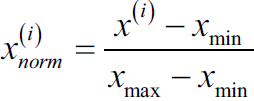
https://blog.csdn.net/Linli522362242/article/details/103587172
Here, is a particular sample, is the smallest value in a feature column, and the largest value.

The min-max scaling procedure is implemented in scikit-learn and can be used as follows:

from sklearn.preprocessing import MinMaxScaler

mms = MinMaxScaler()
X_train_norm = mms.fit_transform(X_train)
X_test_norm = mms.transform(X_test)

min-max scaling VS standardization

Although normalization via min-max scaling is a commonly used technique that is useful when we need values in a bounded interval, standardization can be more practical for many machine learning algorithms, especially for optimization algorithms such as gradient descent. The reason is that many linear models, such as the logistic regression and SVM that we remember from Chapter 3, A Tour of Machine Learning Classifiers Using scikit-learn, initialize the weights to 0 or small random values close to 0. Using standardization, we center the feature columns at mean 0 with standard deviation 1 so that the feature columns takes the form of a normal distribution, which makes it easier to learn the weights. Furthermore, standardization maintains useful information about outliers and makes the algorithm less sensitive to them in contrast to min-max scaling, which scales the data to a limited range of values.

The procedure for standardization can be expressed by the following equation: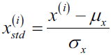

Here, is the sample mean of a particular feature column and the corresponding standard deviation, respectively.

The following table illustrates the difference between the two commonly used feature scaling techniques, standardization and normalization, on a simple sample dataset consisting of numbers 0 to 5:

You can perform the standardization and normalization shown in the table manually by executing the following code examples:

Please note that pandas uses ddof=1 (sample standard deviation) by default,
whereas NumPy's std method and the StandardScaler uses ddof=0 (population standard deviation)
cp1_Journey from Statistics to Machine Learning： https://blog.csdn.net/Linli522362242/article/details/91037961

Numpy's std uses ddof=0 (population standard deviation)

ex = np.array([0,1,2,3,4,5])
print( 'standardized:', ( ex - ex.mean() )/ex.std() )

Panda's std uses ddof=1 (sample standard deviation)

exDF=pd.DataFrame(ex)
print('standardized: ', 
      ( (exDF - exDF.mean())/ exDF.std() ).values.reshape(1, -1)[0]
     )

print('normalized:', 
      ( ex-ex.min() )/( ex.max()-ex.min() )
     )

Similar to the MinMaxScaler class, scikit-learn also implements a class for standardization:

uses ddof=1 (sample standard deviation)

from sklearn.preprocessing import StandardScaler
stdsc = StandardScaler()
print( 'standardized:', 
      stdsc.fit_transform( ex.reshape(-1, 1) ).reshape(1,-1)[0] 
     )

from sklearn.preprocessing import StandardScaler
stdsc = StandardScaler()
X_train_std = stdsc.fit_transform(X_train)
X_test_std = stdsc.transform(X_test)

Again, it is also important to highlight that we fit the StandardScaler class only once—on the training data—and use those parameters to transform the test set or any new data point.

Selecting meaningful features

If we notice that a model performs much better on a training dataset than on the test dataset, this observation is a strong indicator of overfitting. As we discussed in Chapter 3, A Tour of Machine Learning Classifiers Using scikit-learn, overfitting
means the model fits the parameters too closely with regard to the particular observations in the training dataset, but does not generalize well to new data, and we say the model has a high variance. The reason for the overfitting is that our model is too complex for the given training data. Common solutions to reduce the generalization error are listed as follows:

Collect more training data
Introduce a penalty for complexity via regularization
Choose a simpler model with fewer parameters
Reduce the dimensionality of the data

Collecting more training data is often not applicable. In Chapter 6, Learning Best Practices for Model Evaluation and Hyperparameter Tuning, we will learn about a useful technique to check whether more training data is helpful at all. In the
following sections, we will look at common ways to reduce overfitting by regularization and dimensionality reduction via feature selection, which leads to simpler models by requiring fewer parameters to be fitted to the data.

L1 and L2 regularization as penalties against model complexity

We recall from cp3 A Tour of ML Classifiers_stratify_bincount_likelihood_logistic regression_odds ratio_decay_L2 scikitlearnhttps://blog.csdn.net/Linli522362242/article/details/96480059, that L2 regularization is one approach to reduce the complexity of a model by penalizing large individual weights, where we defined the L2 norm of our weight vector w as follows: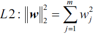

Another approach to reduce the model complexity is the related L1 regularization: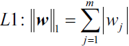

Here, we simply replaced the square of the weights by the sum of the absolute values of the weights. In contrast to L2 regularization, L1 regularization usually yields sparse[spɑrs] feature vectors; most feature weights will be zero. Sparsity['spɑ:sɪtɪ] can be useful in practice if we have a high-dimensional dataset with many features that are irrelevant[ɪˈreləvənt] especially cases where we have more irrelevant dimensions than samples. In this sense, L1 regularization can be understood as a technique for feature selection.

A geometric interpretation of L2 regularization

As mentioned in the previous section, L2 regularization adds a penalty term to the cost function that effectively results in less extreme weight values compared to a model trained with an unregularized cost function. To better understand how L1 regularization encourages sparsity, let's take a step back and take a look at a geometric interpretation of regularization. 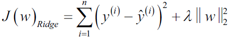Let us plot the contours of a convex cost function for two weight coefficients and . Here, we will consider the Sum of Squared Errors (SSE) cost function that we used for Adaline in Chapter 2, Training Simple Machine Learning Algorithms for Classification, since it is spherical [ˈsfɪrɪkəl, ˈsfɛr-] and easier to draw than the cost function of logistic regression; however, the same concepts apply to the latter. Remember that our goal is to find the combination of weight coefficients that minimize the cost function for the training data, as shown in the following figure (the point in the center of the ellipses):

Now, we can think of regularization as adding a penalty term to the cost function to encourage smaller weights; or, in other words, we penalize large weights.

Thus, by increasing the regularization strength via the regularization parameter , we shrink the weights towards zero and decrease the dependence of our model on the training data. Let's illustrate this concept in the following figure for the L2 penalty term.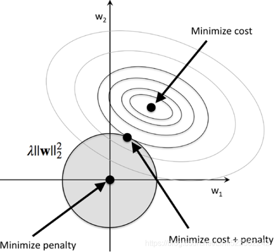
04_TrainingModels_02_regularization_L2_cost_Ridge_Lasso_Elastic Net_Early Stopping: https://blog.csdn.net/Linli522362242/article/details/104070847
The quadratic L2 regularization term is represented by the shaded ball. Here, our weight coefficients cannot exceed our regularization budget—the combination of the weight coefficients###W=w1, w2, w3...wn### cannot fall outside the shaded area. On the other hand, we still want to minimize the cost function(such as The term is just added for our convenience https://blog.csdn.net/Linli522362242/article/details/96480059). Under the penalty constraint, our best effort is to choose the point where the L2 ball intersects with the contours of the unpenalized cost function. The larger the value of the regularization parameter gets, the faster the penalized cost functiongrows, which leads to a narrower L2 ball. For example, if we increase the regularization parameter towards infinity, the weight coefficients will become effectively zero, denoted by the center of the L2 ball. To summarize the main message of the example: our goal is to minimize the sum of the unpenalized cost function plus the penalty term, which can be understood as adding bias and preferring a simpler model to reduce the variance(try to underfit) in the absence of sufficient training data to fit the model.

Now let's discuss L1 regularization and sparsity. The main concept behind L1 regularization is similar to what we have discussed here. However, since the L1 penalty is the sum of the absolute weight coefficients (remember that the L2 term is quadratic), we can represent it as a diamond shape budget, as shown in the following figure:

In the preceding figure, we can see that the contour of the cost function touches the L1 diamond at . Since the contours of an L1 regularized system are sharp, it is more likely that the optimum—that is, the intersection between the ellipses of the cost function and the boundary of the L1 diamond—is located on the axes, which encourages sparsity. The mathematical details of why L1 regularization can lead to sparse solutions are beyond the scope of this book. If you are interested, an excellent section on L2 versus L1 regularization can be found in section 3.4 of The Elements of Statistical Learning, Trevor Hastie, Robert Tibshirani, and Jerome Friedman, Springer.

For regularized models in scikit-learn that support L1 regularization, we can simply set the penalty parameter to 'l1' to yield the sparse solution:

from sklearn.linear_model import LogisticRegression

LogisticRegression(penalty='l1', solver='liblinear', multi_class='ovr')

Applied to the standardized Wine data, the L1 regularized logistic regression would yield the following sparse solution

Note that C=1.0 is the default. You can increase or decrease it to make the regulariztion effect stronger or weaker, respectively.

from sklearn.linear_model import LogisticRegression

lr = LogisticRegression(penalty='l1', C=1.0, solver='liblinear', multi_class='ovr')
lr.fit(X_train_std, y_train)
print('Training accuracy:', lr.score(X_train_std, y_train))
print('Test accuracy: ', lr.score(X_test_std, y_test))

Both training and test accuracies (both 100 percent) indicate that our model does a perfect job on both datasets. When we access the intercept terms via the lr.intercept_ attribute, we can see that the array returns three values:

lr.intercept_

# since 3 classes # w0

np.unique( y_train )

Since we fit the LogisticRegression object on a multiclass dataset, it uses the Oneversus-Rest (OvR) approach by default, where the first intercept belongs to the model that fits class 1 versus class 2 and 3, the second value is the intercept of the
model that fits class 2 versus class 1 and 3, and the third value is the intercept of the model that fits class 3 versus class 1 and 2:

lr.coef_

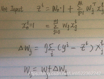
The weight array that we accessed via the lr.coef_ attribute contains three rows of weight coefficients, one weight vector for each class. Each row consists of 13 weights where each weight is multiplied by the respective feature in the 13-dimensional Wine dataset to calculate the net input:

########################################################################

np.sum(lr.coef_, axis=0)!=0.

df_wine.columns[1:][np.sum(lr.coef_, axis=0)!=0.]

df_wine.columns[1:][np.sum(lr.coef_, axis=0)==0.]

these columns we may drop ?:

Is it possible to drop some feature columns based on the weight coefficient (if the coefficient value is 0)？https://blog.csdn.net/Linli522362242/article/details/108272169

the answer is No:

########################################################################

Note
In scikit-learn, corresponds to the intercept_ and with correspond to the values in coef_.

As a result of L1 regularization, which serves as a method for feature selection, we just trained a model that is robust to the potentially irrelevant features in this dataset.

Strictly speaking, the weight vectors from the previous example are not necessarily sparse, though, because they contain more non-zero than zero entries. However, we could enforce sparsity (more zero entries) by further increasing the regularization strength—that is, choosing lower values for the C parameter(higher value ).

In the last example on regularization in this chapter, we will vary the regularization strength and plot the regularization path—the weight coefficients of the different features for different regularization strengths:

import matplotlib.pyplot as plt

fig = plt.figure()
ax = plt.subplot(111)

colors = ['blue', 'green', 'red', 'cyan', 
          'magenta', 'yellow', 'black', 
          'pink', 'lightgreen', 'lightblue', 
          'gray', 'indigo', 'orange']

weights, params = [], []

for c in np.arange(-4., 6.):
    lr = LogisticRegression( penalty='l1', C=10.**c, solver='liblinear', multi_class='ovr', random_state=0 )
    lr.fit(X_train_std, y_train)
    weights.append(lr.coef_[1])
    params.append(10**c)

weights = np.array(weights)
                                #features
for column, color in zip( range(weights.shape[1]), colors):
    plt.plot( params, weights[:, column], label=df_wine.columns[column+1], color=color )# +1 since [0] is 'Class label'

plt.axhline(0, color='black', linestyle='--', linewidth=3)
plt.xlim([10**(-5), 10**5])
plt.ylabel('Weight Coefficient')
plt.xlabel('C')
plt.xscale('log')######
           
#          loc: legend box's corner as the anchor point
ax.legend( loc='upper left',bbox_to_anchor=(1.04, 1.03), # anchor point's location: ( h_x==>left, v_y==>up )
           ncol=1, fancybox=True )                       # from current plot's lower-upper corner

plt.show()

The resulting plot provides us with further insights into the behavior of L1 regularization. As we can see, all feature weights will be zero if we penalize the model with a strong regularization parameter ( ); C is the inverse of the regularization parameter :

Sequential feature selection algorithms

https://blog.csdn.net/Linli522362242/article/details/108272169

cp4 Training Sets Preprocessing_StringIO_dropna_categorical_feature_Encode_Scale_L1_L2_bbox_to_ancho