LDA是一种以目标:
- 类重心点距离最大
- 类内点距离小
但是对于情况:两个类重心点很近,但是各个点距离很远的情况,适用性不好。下面举个例子。
1、数据生成
首先建立一个函数
%生成一系列园点
function [x1,y1] = creat_circle(r1 , r1_ratio,sita_ratio)
sita = 0:0.05:2*pi;
all_num = size(sita);
all_num = all_num(1,2);
%rand : sita
sita_p = randperm(all_num,floor(sita_ratio*all_num));
%rand : r
r_p = rand(1,floor(sita_ratio*all_num))*r1*r1_ratio;
r1_p = repmat(r1,1,floor(sita_ratio*all_num));
r1_p = r1_p - r_p;
x1 = r1_p.*cos(sita_p);
y1 = r1_p.*sin(sita_p);
scatter(x1,y1)
然后使用程序(matlab)
clear;clc;close all;
[x1,y1] = creat_circle(3,0.05,0.95);
[x2,y2] = creat_circle(5,0.05,0.95);
[x3,y3] = creat_circle(9,0.05,0.95);
num = size(x1);
z1 = normrnd(5,1,1,num(1,2))+x1;
z2 = wgn(1,num(1,2),1)+4+y2;
z3 = rand(1,num(1,2))+2+x3;
% 画
figure(1)
scatter(x1,y1,'r')
hold on
scatter(x2,y2,'b')
scatter(x3,y3,'g')
figure(2)
scatter3(x1,y1,z1,'r')
hold on
scatter3(x2,y2,z2,'b');
scatter3(x3,y3,z3,'g');
可以看出数据点的分布:

显然是有规律的(类似行星环)
但是进过LDA降维(降至2维)就失去了特性。
2、LDA降维
首先从网上查了一个LDA函数:
function [mappedX, mapping] = FisherLDA(X, labels, no_dims)
%LDA Perform the LDA algorithm
%
%   [mappedX, mapping] = lda(X, labels, no_dims)
%
% The function runs LDA on a set of datapoints X. The variable
% no_dims sets the number of dimensions of the feature points in the
% embedded feature space (no_dims >= 1, default = 2). The maximum number
% for no_dims is the number of classes in your data minus 1.
% The function returns the coordinates of the low-dimensional data in
% mappedX. Furthermore, it returns information on the mapping in mapping.
%
%

% This file is part of the Matlab Toolbox for Dimensionality Reduction.
% The toolbox can be obtained from http://homepage.tudelft.nl/19j49
% You are free to use, change, or redistribute this code in any way you
% want for non-commercial purposes. However, it is appreciated if you
% maintain the name of the original author.
%
% (C) Laurens van der Maaten, Delft University of Technology


    if ~exist('no_dims', 'var') || isempty(no_dims)
        no_dims = 2;
    end

	% Make sure data is zero mean
    mapping.mean = mean(X, 1);
	X = bsxfun(@minus, X, mapping.mean);

	% Make sure labels are nice
	[classes, bar, labels] = unique(labels);
    nc = length(classes);

	% Intialize Sw
	Sw = zeros(size(X, 2), size(X, 2));

    % Compute total covariance matrix
    St = cov(X);

	% Sum over classes
	for i=1:nc

        % Get all instances with class i
        cur_X = X(labels == i,:);

		% Update within-class scatter
		C = cov(cur_X);
		p = size(cur_X, 1) / (length(labels) - 1);
		Sw = Sw + (p * C);
    end

    % Compute between class scatter
    Sb = St - Sw;
    Sb(isnan(Sb)) = 0; Sw(isnan(Sw)) = 0;
	Sb(isinf(Sb)) = 0; Sw(isinf(Sw)) = 0;

    % Make sure not to embed in too high dimension
    if nc <= no_dims
        no_dims = nc - 1;
        warning(['Target dimensionality reduced to ' num2str(no_dims) '.']);
    end

	% Perform eigendecomposition of inv(Sw)*Sb
    [M, lambda] = eig(Sb, Sw);

    % Sort eigenvalues and eigenvectors in descending order
    lambda(isnan(lambda)) = 0;
	[lambda, ind] = sort(diag(lambda), 'descend');
	M = M(:,ind(1:min([no_dims size(M, 2)])));

	% Compute mapped data
	mappedX = X * M;

    % Store mapping for the out-of-sample extension
    mapping.M = M;
    mapping.val = lambda;
然后运行总代码:
% 建立坐标点
clear;clc;close all;
[x1,y1] = creat_circle(3,0.05,0.95);
[x2,y2] = creat_circle(5,0.05,0.95);
[x3,y3] = creat_circle(9,0.05,0.95);
num = size(x1);
z1 = normrnd(5,1,1,num(1,2))+x1;
z2 = wgn(1,num(1,2),1)+4+y2;
z3 = rand(1,num(1,2))+2+x3;
% 画
figure(1)
scatter(x1,y1,'r')
hold on
scatter(x2,y2,'b')
scatter(x3,y3,'g')
figure(2)
scatter3(x1,y1,z1,'r')
hold on
scatter3(x2,y2,z2,'b');
scatter3(x3,y3,z3,'g');
X = [x1,x2,x3];
Y = [y1,y2,y3];
Z = [z1,z2,z3];
data = [X;Y;Z]';
label_11 = zeros(size(x1))+1;
label_2 = zeros(size(x2))+2;
label_3 = zeros(size(x3))+3;
labels = [label_11,label_2,label_3];
[mappedX, ~] = FisherLDA(data, labels, 2);
figure(2)
hold on
axis equal
scatter(mappedX(1:119,1),mappedX(1:119,2),'r*')
scatter(mappedX(2:238,1),mappedX(2:238,2),'b')
scatter(mappedX(239:357,1),mappedX(239:357,2),'g')
figure(3)
scatter(mappedX(:,1),mappedX(:,2),'b')
得到了降维后的图
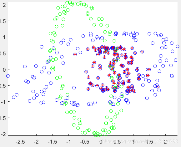
完全失去了规律