目录
Matplotlib 是建立在NumPy基础之上的Python绘图库,是在机器学习中用于数据可视化的工具
Matplotlib具有很强的工具属性,也就是说它只是为我所用的,我们不必花太多的精力去精进它。
我们只需要知道它可以做哪些事,可以绘制哪些图形,有一个印象就足够了。
我们在实际使用中用什么拿什么,我们用到了自然就熟练了。
一、Matplotlib常见用法
1. 绘制简单图像
我们以机器学习中最常见的激活函数sigmoid举例,我们来绘制它。
import matplotlib.pyplot as plt
import numpy as np
x = np.linspace(-10,10,1000)
y = 1 / (1 + np.exp(-x))
plt.plot(x,y)
plt.show()
其中sigmoid的公式为:
plot()方法展示变量间的趋势,show()方法展示图像。
我们得到如图所示图像:

2. 添加常用元素
我们添加一些参考元素,各函数的解释我在代码中进行了详细的标注。
x = np.linspace(-10,10,1000)

#写入公式
y = 1 / (1 + np.exp(-x))

#x轴范围限制
plt.xlim(-5,5)

#y轴范围限制
plt.ylim(-0.2,1.2)

#x轴添加标签
plt.xlabel("X axis")

#y轴添加标签
plt.ylabel("Y axis")

#标题
plt.title("sigmoid function")

#设置网格,途中红色虚线
plt.grid(linestyle=":", color ="red")

#设置水平参考线
plt.axhline(y=0.5, color="green", linestyle="--", linewidth=2)

#设置垂直参考线
plt.axvline(x=0.0, color="green", linestyle="--", linewidth=2)

#绘制曲线
plt.plot(x,y)

#保存图像
plt.savefig("./sigmoid.png",format='png', dpi=300)
以上代码包含了限制X、Y轴范围,添加标题和标签,设置网格,添加参考线,保存图像等内容。
绘制图像如下:

3. 绘制多曲线
#生成均匀分布的1000个数值
x = np.linspace(-10,10,1000)

#写入sigmoid公式
y = 1 / (1 + np.exp(-x))
z = x**2
plt.xlim(-2,2)
plt.ylim(0,1)

#绘制sigmoid
plt.plot(x,y,color='#E0BF1D',linestyle='-', label ="sigmoid")

#绘制y=x*x
plt.plot(x,z,color='purple',linestyle='-.', label = "y=x*x")

#绘制legend,即下图角落的图例
plt.legend(loc="upper left")

#展示
plt.show()
绘制多图像直接调用多个plot()即可。
注意:如果不调用legend()方法,不会绘制左上角的legend(图例)。其中color参数支持hex表示。

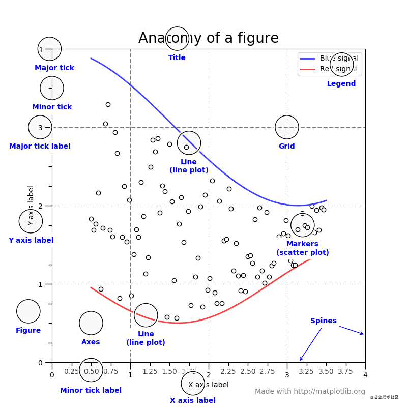
4. 认识figure(画布)
首先我们认识figure(画布),比如legend我们在上文中提到过,是线条标签的展示。
grid所圈住的虚线是网格参考线。Title/x axislabel等文本标签。这张图有助于我们对figure有一个直观的理解。
5. 绘制多图像
一个figure是可以对应多个plot的,现在我们试着在一个figure上绘制多图像。
x = np.linspace(-2*np.pi, 2*np.pi, 400)
y = np.sin(x**2)
z = 1 / (1 + np.exp(-x))
a = np.random.randint(0,100,400)
b = np.maximum(x,0.1*x)

#创建两行两列的子图像
fig, ax_list = plt.subplots(nrows=2, ncols=2)

# 'r-'其中r表示color=red,-表示linestyle='-'
ax_list[0][0].plot(x,y,'r-')
ax_list[0][0].title.set_text('sin')

ax_list[0][1].scatter(x,a,s=1)
ax_list[0][1].title.set_text('scatter')

ax_list[1][0].plot(x,b,'b-.')
ax_list[1][0].title.set_text('leaky relu')

ax_list[1][1].plot(x,z,'g')
ax_list[1][1].title.set_text('sigmoid')

#调整子图像的布局
fig.subplots_adjust(wspace=0.9,hspace=0.5)
fig.suptitle("Figure graphs",fontsize=16)
plt.show()
其中,最关键的是subplots方法,生成2行2列的子图像,然后我们调用ax_list中的各绘图方法。
其中'r-','b-.'参数为绘图的缩写写法,本文后续参数缩写段落会单独讲解。

6. 绘制常用图
我们常用图来表示数据之间的关系,常见的图包括直方图、柱状图、饼图、散点图等等。
# import matplotlib.pyplot as plt
# import numpy as np
# x = np.linspace(-10,10,100)
# y = 1 / (1+np.exp(-x))
# plt.plot(x,y);
# plt.show()

#添加一些参考元素
# import numpy as np
# import matplotlib.pyplot as plt
# x = np.linspace(-10,10,1000)
# y = 1/ (1+np.exp(-x))
# #x轴范围限制
# plt.xlim(-5,5)
# #y轴范围限制
# plt.ylim(-0.2,1.2)
# # x轴添加标签
# plt.xlabel("X axis")
# #y轴添加标签
# plt.ylabel("Y axis")
# #标题
# plt.title("Sigmoid function")
#
# # 设置网格,途中红色虚线
# plt.grid(linestyle = ":",color = "red")
#
# # 设置水平参考线
# plt.axhline(y=0.5,color="green",linestyle="--",linewidth=2)
# #设置垂直参考线
# plt.axvline(x =0.0,color="green",linestyle="--",linewidth=2)
# #绘制曲线
# plt.plot(x,y)
# plt.show()
# #保存图像
# # plt.savefig("./sigmod.png",format="png",dpi=300)
#

#绘制多曲线
# import numpy as np
# import matplotlib.pyplot as plt
# #生成均匀分布的1000个数值
# x = np.linspace(-10,10,1000)
# y = 1/(1+np.exp(-x))
# z = x**2;
# plt.xlim(-2,2)
# plt.ylim(0,1)
# #绘制sigmod
# plt.plot(x,y,color="red",linestyle="-",label="sigmod")
# #绘制y = x**2
# plt.plot(x,z,color="purple",linestyle="-.",label="y=x**2")
# plt.legend(loc="upper left") #左上方角落的图例。
# plt.show()


# 绘制多图像
#一个figure是可以对应多个plot的
# import numpy as np
# import matplotlib.pyplot as plt
# x = np.linspace(-2*np.pi,2*np.pi,400)
# y = np.sin(x**2)
# z = 1/(1+np.exp(-x))
# a = np.random.randint(0,100,400)
# b = np.maximum(x,0.1*x)
# #创建两行两列的子对象
# fig ,ax_list = plt.subplots(nrows =2,ncols =2)
# # r-中r表示color = red. - 表示linestyle ='-'
# ax_list[0][0].plot(x,y,"r-")
# ax_list[0][0].title.set_text("scatter")
#
# ax_list[0][1].scatter(x,a,s=1)
# ax_list[0][1].title.set_text('scatter')
#
# ax_list[1][0].plot(x,b,'b-.')
# ax_list[1][0].title.set_text('leaky relu')
#
# ax_list[1][1].plot(x,z,'g')
# ax_list[1][1].title.set_text('sigmoid')
#
# fig.subplots_adjust(wspace=0.9,hspace=0.5)
# fig.suptitle("Figure graphs",fontsize = 16)
# fig.show()
# plt.show()
#
#

# 绘制常用图
#直方图,柱状图,饼图,散点图等
# 使绘图支持中文
import numpy as np
import matplotlib.pyplot as plt

plt.rcParams['font.sans-serif'] = ['Arial Unicode MS']

#plt.rcParams["font.sans_serif"]=["Microsoft YaHei"]
#创建两行两列的子对象
fig,[[ax1,ax2],[ax3,ax4],[ax5,ax6]]=plt.subplots(nrows=3,ncols=2,figsize=(8,8))
#绘制柱状图
value = (2,3,4,1,2)
index = np.arange(5)
ax1.bar(index,value,alpha = 0.4,color="b")
ax1.set_xlabel("Group")
ax1.set_ylabel("Scores")
ax1.set_title("柱状图")

#绘制直方图
h = 100 + 15*np.random.randn(437)
ax2.hist(h,bins=50)
ax2.title.set_text("直方图")

#绘制饼图pie
labels = "Frogs","CAT","yongji","Logs"
sizes =[15,30,45,10]
explode =(0,0.1,0,0)
ax3.pie(sizes,explode = explode,labels=labels,autopct='%1.1f%%',
        shadow = True,startangle = 90)
ax3.axis("equal")
ax3.title.set_text("饼图")

# 绘制棉棒图
x = np.linspace(0.5,2*np.pi,20)
y = np.random.randn(20)
ax4.stem(x,y,linefmt="-",markerfmt ="o",basefmt='-')
ax4.title.set_text("棉棒图")
#绘制气泡图scatter
a = np.random.randn(100)
b = np.random.randn(100)
ax5.scatter(a,b,s=np.power(2*a+4*b,2),c = np.random.rand(100),cmap=plt.cm.RdYlBu,marker='o')

#绘制极线图polar
fig.delaxes(ax6)
ax6 = fig.add_subplot(236,projection='polar')
r = np.arange(0,2,0.01)
theta = 2*np.pi*r
ax6.plot(theta,r)
ax6.set_rmax(2)
ax6.set_rticks([0.5,1,1.5,2])
ax6.set_rlabel_position(-22.5)
ax6.grid(True)
#调整子图像的布局
fig.subplots_adjust(wspace=1,hspace=1.2)
fig.suptitle("图形绘制", fontsize=16)
plt.show()
绘制图像如下:

7. 参数简写
因为matplotlib支持参数的缩写,所以我认为有必要单独拿出来讲一讲各参数缩写的表示。
x = np.linspace(-10,10,20)
y = 1 / (1 + np.exp(-x))
plt.plot(x,y,c='k',ls='-',lw=5, label ="sigmoid", marker="o", ms=15, mfc='r')
plt.legend()
plt.show()
绘制图像如下:

7.1 c代表color(颜色)
| 字符 | 颜色 |
|---|---|
| ‘b’ | blue |
| ‘g’ | green |
| ‘r’ | red |
| ‘c’ | cyan |
| ‘m’ | magenta |
| ‘y’ | yellow |
| ‘k’ | black |
| ‘w’ | white |
7.2 ls代表linestyle(线条样式)
| 字符 | 描述 |
|---|---|
| '-' | solid line style |
| '--' | dashed line style |
| '-.' | dash-dot line style |
| ':' | dotted line style |
| '.' | point marker |
| ',' | pixel marker |
| 'o' | circle marker |
| 'v' | triangle_down marker |
| '^' | triangle_up marker |
| '<' | triangle_left marker |
| '>' | triangle_right marker |
| '1' | tri_down marker |
| '2' | tri_up marker |
| '3' | tri_left marker |
| '4' | tri_right marker |
| 's' | square marker |
| 'p' | pentagon marker |
| '*' | star marker |
| 'h' | hexagon1 marker |
| 'H' | hexagon2 marker |
| '+' | plus marker |
| 'x' | x marker |
| 'D' | diamond marker |
| 'd' | thin_diamond marker |
| '|' | vline marker |
| '_' | hline marker |
7.3 marker(记号样式)
记号样式展示如下: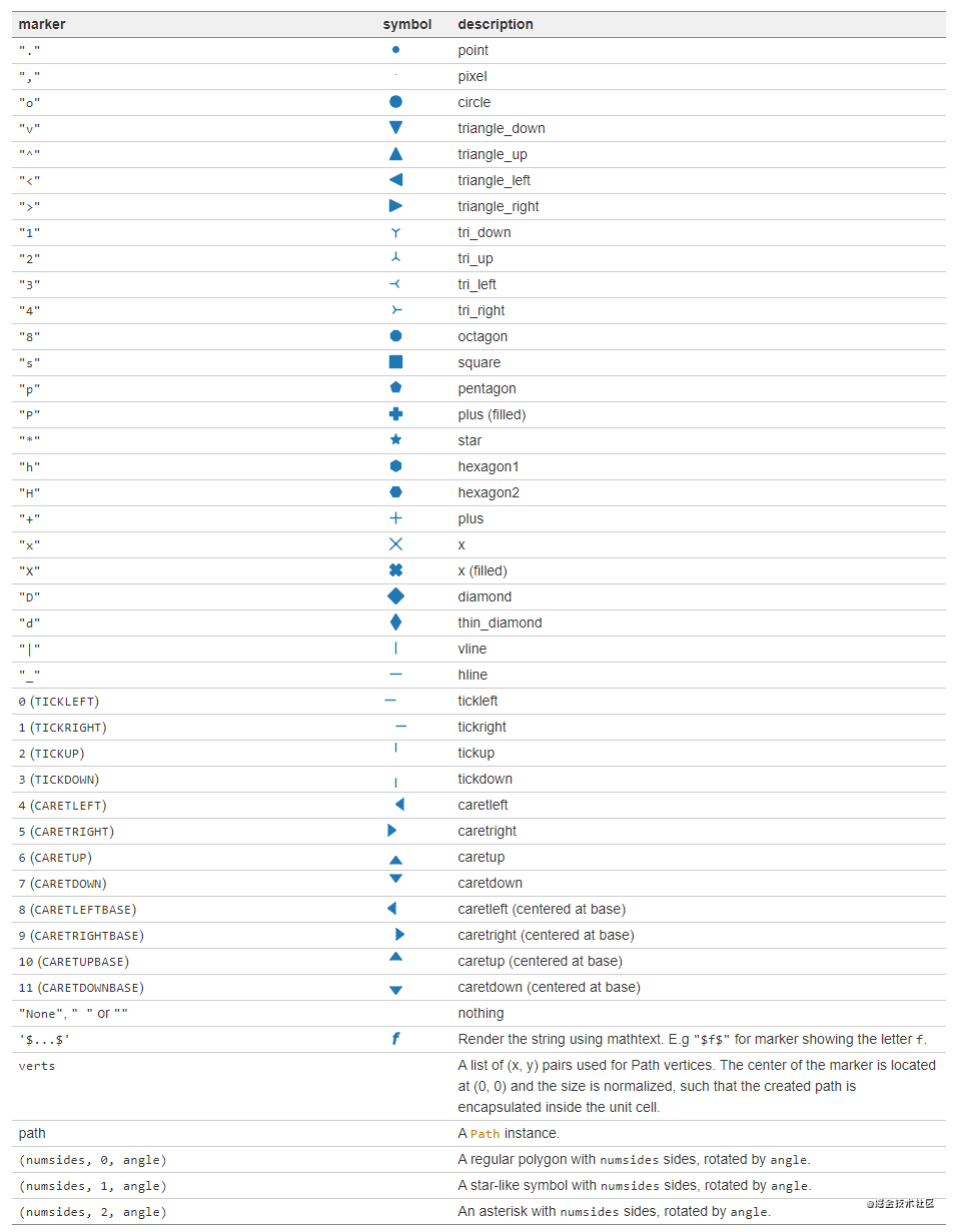
7.4 其他缩写
-
lw代表linewidth(线条宽度),如:lw=2.5 -
ms代表markersize(记号尺寸),如:ms=5 -
mfc代表markerfacecolor(记号颜色),如:mfc='red'
二、Matplotlib进阶用法
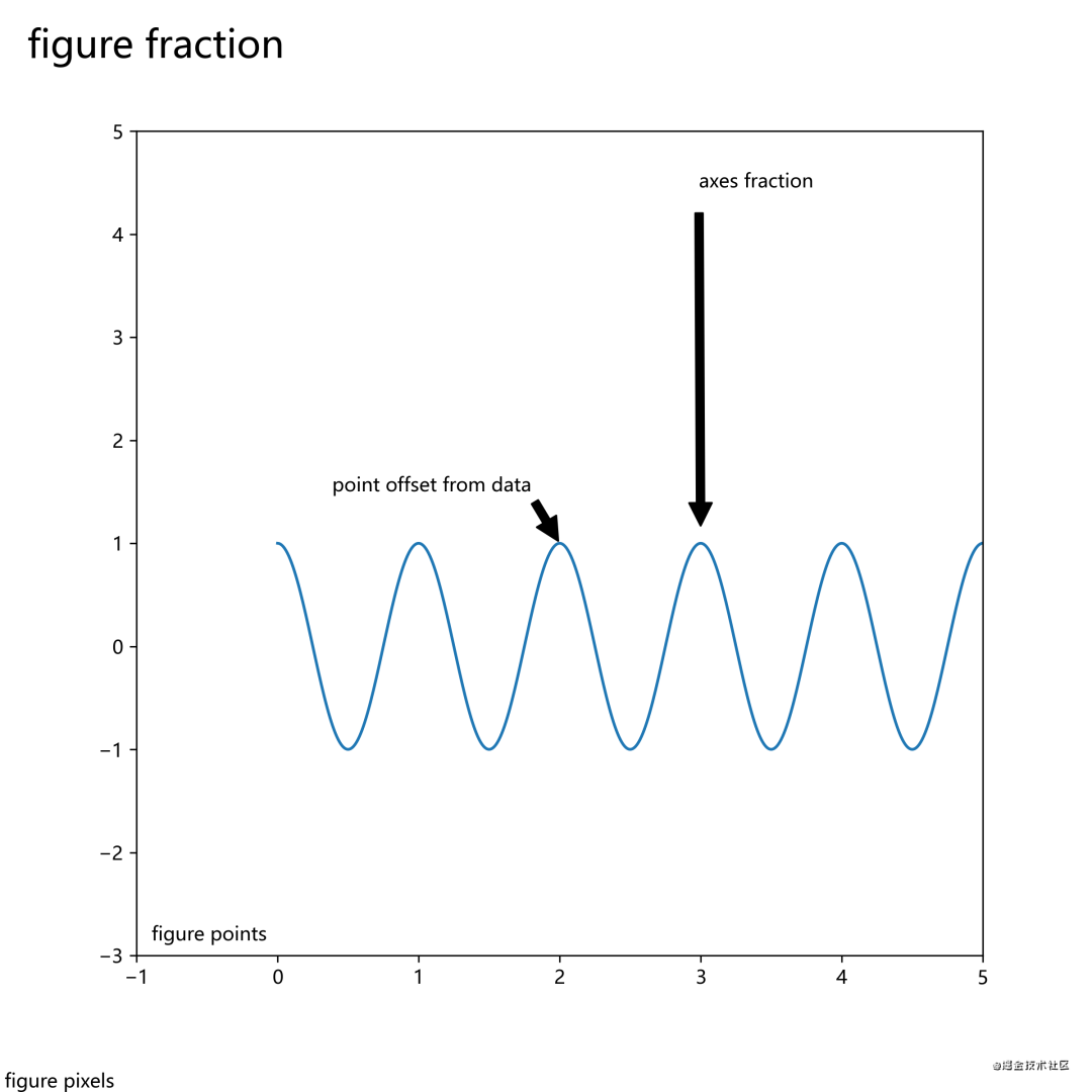
1. 添加文本注释
我们可以在画布(figure)上添加文本、箭头等标注,来让图像表述更清晰准确。
我们通过调用annotate方法来绘制注释。
fig, ax = plt.subplots(figsize=(8, 8))

t = np.arange(0.0, 5.0, 0.01)
s = np.cos(2*np.pi*t)

# 绘制一条曲线
line, = ax.plot(t, s)

#添加注释
ax.annotate('figure pixels',
            xy=(10, 10), xycoords='figure pixels')
ax.annotate('figure points',
            xy=(80, 80), xycoords='figure points')
ax.annotate('figure fraction',
            xy=(.025, .975), xycoords='figure fraction',
            horizontalalignment='left', verticalalignment='top',
            fontsize=20)

#第一个箭头
ax.annotate('point offset from data',
            xy=(2, 1), xycoords='data',
            xytext=(-15, 25), textcoords='offset points',
            arrowprops=dict(facecolor='black', shrink=0.05),
            horizontalalignment='right', verticalalignment='bottom')

#第二个箭头
ax.annotate('axes fraction',
            xy=(3, 1), xycoords='data',
            xytext=(0.8, 0.95), textcoords='axes fraction',
            arrowprops=dict(facecolor='black', shrink=0.05),
            horizontalalignment='right', verticalalignment='top')

ax.set(xlim=(-1, 5), ylim=(-3, 5))
绘制图像如下:
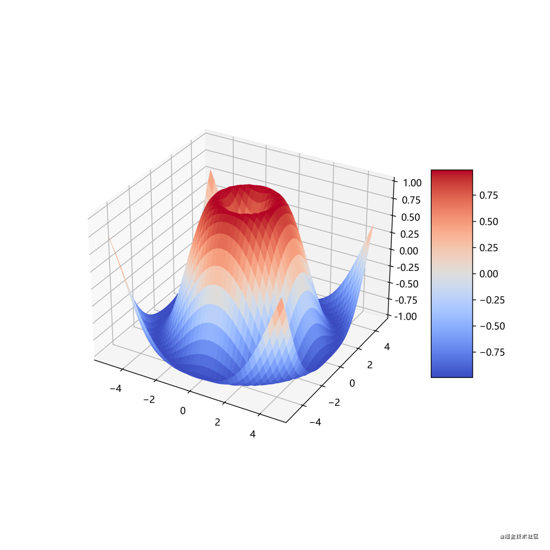
2. 绘制3D图像
绘制3D图像需要导入Axes3D库。
from mpl_toolkits.mplot3d import Axes3D
import matplotlib.pyplot as plt
from matplotlib import cm
from matplotlib.ticker import LinearLocator, FormatStrFormatter
import numpy as np


fig = plt.figure(figsize=(15,15))
ax = fig.gca(projection='3d')

# Make data.
X = np.arange(-5, 5, 0.25)
Y = np.arange(-5, 5, 0.25)
X, Y = np.meshgrid(X, Y)
R = np.sqrt(X**2 + Y**2)
Z = np.sin(R)

# Plot the surface.
surf = ax.plot_surface(X, Y, Z, cmap=cm.coolwarm,
                       linewidth=0, antialiased=False)

# Customize the z axis.
ax.set_zlim(-1.01, 1.01)
ax.zaxis.set_major_locator(LinearLocator(10))
ax.zaxis.set_major_formatter(FormatStrFormatter('%.02f'))

# Add a color bar which maps values to colors.
fig.colorbar(surf, shrink=0.5, aspect=5)
其中cmap意为colormap,用来绘制颜色分布、渐变色等。cmap通常配合colorbar使用,来绘制图像的颜色栏。
3. 导入图像(加州房价)
引入mpimg库,来导入图像。
我们以美国加州房价数据为例,导入加州房价数据绘制散点图,同时导入加州地图图片,查看地图经纬度对应房价的数据。同时使用颜色栏,绘制热度图像。
代码如下:
import os
import urllib
import numpy as np
import pandas as pd
import matplotlib.pyplot as plt
import matplotlib.image as mpimg

#加州房价数据(大家不用在意域名)
housing = pd.read_csv("http://blog.caiyongji.com/assets/housing.csv")
#加州地图
url = "http://blog.caiyongji.com/assets/california.png"
urllib.request.urlretrieve("http://blog.caiyongji.com/assets/california.png", os.path.join("./", "california.png"))
california_img=mpimg.imread(os.path.join("./", "california.png"))

#根据经纬度绘制房价散点图
ax = housing.plot(kind="scatter", x="longitude", y="latitude", figsize=(10,7),
                       s=housing['population']/100, label="Population",
                       c="median_house_value", cmap=plt.get_cmap("jet"),
                       colorbar=False, alpha=0.4,
                      )
plt.imshow(california_img, extent=[-124.55, -113.80, 32.45, 42.05], alpha=0.5,
           cmap=plt.get_cmap("jet"))
plt.ylabel("Latitude", fontsize=14)
plt.xlabel("Longitude", fontsize=14)

prices = housing["median_house_value"]
tick_values = np.linspace(prices.min(), prices.max(), 11)

#颜色栏,热度地图
cbar = plt.colorbar(ticks=tick_values/prices.max())
cbar.ax.set_yticklabels(["$%dk"%(round(v/1000)) for v in tick_values], fontsize=14)
cbar.set_label('Median House Value', fontsize=16)
v
plt.legend(fontsize=16)
绘制图像如下:
红色昂贵,蓝色便宜,圆圈大小表示人口多少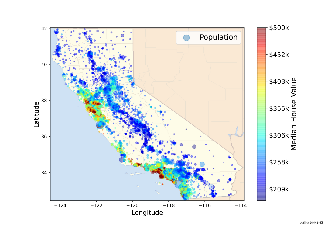
4. 绘制等高线
等高线对于在二维空间内绘制三维图像很有用。
def f(x, y):
    return np.sin(x) ** 10 + np.cos(10 + y * x) * np.cos(x)

x = np.linspace(0, 5, 50)
y = np.linspace(0, 5, 40)

X, Y = np.meshgrid(x, y)
Z = f(X, Y)
plt.contourf(X, Y, Z, 20, cmap='RdGy')
plt.colorbar()
绘制图像如下:
黑色地方是峰,红色地方是谷。

绘制动画
绘制动画需要引入animation库,通过调用FuncAnimation方法来实现绘制动画。
import numpy as np
from matplotlib import pyplot as plt
from matplotlib import animation

fig = plt.figure()
ax = plt.axes(xlim=(0, 2), ylim=(-2, 2))
line, = ax.plot([], [], lw=2)

# 初始化方法
def init():
    line.set_data([], [])
    return line,

# 数据更新方法,周期性调用
def animate(i):
    x = np.linspace(0, 2, 1000)
    y = np.sin(2 * np.pi * (x - 0.01 * i))
    line.set_data(x, y)
    return line,

#绘制动画,frames帧数,interval周期行调用animate方法
anim = animation.FuncAnimation(fig, animate, init_func=init,
                               frames=200, interval=20, blit=True)
anim.save('ccccc.gif', fps=30)

plt.show()
上述代码中anim.save()方法支持保存mp4格式文件。
绘制动图如下: