统计学习方法2 - 感知机

感知机：判别模型、二分类线性模型
模型形式：
$f(x)=sign(w\cdot x+b)$
$w$ 和 $b$ 为感知机模型参数， $s i g n$ 是符号函数。
要求：数据集线性可分
目的：求将数据集线性划分为两部分的超平面
经验损失函数：所有误分类的点到超平面距离之和 $L (w, b)$
极小化经验损失函数方法：梯度下降法
算法流程：
- 输入：训练数据集 $\begin{Bmatrix} (x_{1},y_{1}),(x_{2},y_{2}),\cdots ,(x_{N},y_{N}) \end{Bmatrix}$ , 学习率 $\eta$
- 输出：w、b以及感知机模型 $f(x)=sign(w\cdot x+b)$
- 第一步：初始化 $w_{0}$ 和 $b_{0}$
- 第二步：在训练集中选择数据 $x_{i},y_{i}$
- 第三步：如果 $y_{i}(w\cdot x_{i}+b)\leq 0$ :
  $w\leftarrow w+\eta y_{i}x_{i}$
  $b\leftarrow b+\eta y_{i}$
- 第四步：转至（2），直到没有误分类点。
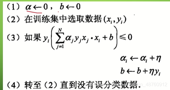
算法对偶
这里每次更新的是误分类的次数 $n_{i}$ ,误分类会导致 $n_{i}$ +1
同时，这里也会有个GRAM举证，是 $x_{i} \cdot x_{j}$ 形成的矩阵， $x_{11} = x_{1} \cdot x_{1}$ ， $x_{12} = x_{1} \cdot x_{2}$ ， $x_{13} = x_{1} \cdot x_{3}$
$x_{21} = x_{2} \cdot x_{1}$ ， $x_{22} = x_{2} \cdot x_{2}$ ， $x_{23} = x_{2} \cdot x_{3}$

参考b站的两个视频，对算法的推导理解比较好：
https://www.bilibili.com/video/BV1Pv411z7J4?from=search&seid=13315330278823399625
https://www.bilibili.com/video/BV14t4y1k7CM

对偶手动迭代可以看看：
https://www.cnblogs.com/qiu-hua/p/12755378.html

课后作业：
习题2.1
Minsky 与 Papert 指出：感知机因为是线性模型，所以不能表示复杂的函数，如异或 (XOR)。验证感知机为什么不能表示异或。

解答：
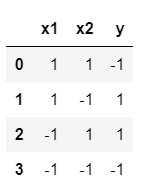
对于异或函数XOR，全部的输入与对应的输出如下：
在这里插入图片描述

%matplotlib inline
import matplotlib.pyplot as plt
import numpy as np
import pandas as pd

x1 = [1, 1, -1, -1]
x2 = [1, -1, 1, -1]
y = [-1, 1, 1, -1]
x1 = np.array(x1)
x2 = np.array(x2)
y = np.array(y)
data = np.c_[x1, x2, y]
data = pd.DataFrame(data, index=None, columns=['x1', 'x2', 'y'])
data.head()

在这里插入图片描述

positive = data.loc[data['y'] == 1]
negative = data.loc[data['y'] == -1]

plt.xlim(-2, 2)
plt.ylim(-2, 2)
plt.xticks([-2, -1, 0, 1, 2])
plt.yticks([-2, -1, 0, 1, 2])
plt.xlabel("x1")
plt.ylabel("x2")
plt.plot(positive['x1'], positive['x2'], "ro")
plt.plot(negative['x1'], negative['x2'], "gx")
plt.show()

在这里插入图片描述
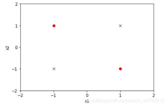
显然感知机无法使用一条直线将两类样本划分，异或问题是线性不可分的。

习题2.2
模仿例题 2.1，构建从训练数据求解感知机模型的例子。
解答：

from sklearn.linear_model import Perceptron
import numpy as np

X_train = np.array([[3, 3], [4, 3], [1, 1]])
y = np.array([1, 1, -1])

perceptron_model = Perceptron()
perceptron_model.fit(X_train, y)
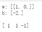
print("w:", perceptron_model.coef_, "\nb:", perceptron_model.intercept_, "\n")

result = perceptron_model.predict(X_train)
print(result)

在这里插入图片描述

统计学习方法2 - 感知机

猜你喜欢