PyTorch(2):搭建神经网络
主要内容是通过Pytorch进行简单神经网络的搭建。
关系拟合(回归) Regression
import torch
import torch.nn.functional as F
import matplotlib.pyplot as plt

x = torch.unsqueeze(torch.linspace(-1,1,100),dim=1)  # x data (tensor),shape=(100,1)
y = x.pow(2) + 0.2*torch.rand(x.size())                 # noisy y data (tensor),shape=(100,1)

class Net(torch.nn.Module):
    def __init__(self,n_feature,n_hidden,n_output):
        super(Net,self).__init__()
        self.hidden = torch.nn.Linear(n_feature,n_hidden)   # hidden layer
        self.predict = torch.nn.Linear(n_hidden,n_output)   # output layer

    def forward(self,x):
        x = F.relu(self.hidden(x))      # activation function for hidden layer
        x = self.predict(x)             # linear output
        return x

net = Net(n_feature=1,n_hidden=10,n_output=1)     # define the network
print(net)  # net architecture

optimizer = torch.optim.SGD(net.parameters(),lr=0.2)  # 随机梯度下降  lr = learning rate
loss_func = torch.nn.MSELoss()  # this is for regression mean squared loss   均方差

plt.ion()   # something about plotting  实时打印配置

for t in range(200):
    prediction = net(x)     # input x and predict based on x

    loss = loss_func(prediction,y)     # must be (1。nn output,2。target)

    optimizer.zero_grad()   # clear gradients for next train
    loss.backward()         # backpropagation,compute gradients
    optimizer.step()        # apply gradients

    if t % 5 == 0:
        # plot and show learning process
        plt.cla()
        plt.scatter(x.data.numpy(),y.data.numpy())
        plt.plot(x.data.numpy(),prediction.data.numpy(),'r-',lw=5)
        plt.text(0.5,0,'Loss=%.4f' % loss.data.numpy(),fontdict={

    'size': 20,'color':  'red'})
        plt.pause(0.1)

plt.ioff()
plt.show()
output:
分类问题(Classification)
import torch
import torch.nn.functional as F
import matplotlib.pyplot as plt

# torch.manual_seed(1)    # reproducible

# make fake data
n_data = torch.ones(100,2)
x0 = torch.normal(2*n_data,1)      # class0 x data (tensor),shape=(100,2)
y0 = torch.zeros(100)               # class0 y data (tensor),shape=(100,1)
x1 = torch.normal(-2*n_data,1)     # class1 x data (tensor),shape=(100,2)
y1 = torch.ones(100)                # class1 y data (tensor),shape=(100,1)
x = torch.cat((x0,x1),0).type(torch.FloatTensor)  # shape (200,2) FloatTensor = 32-bit floating  数据
y = torch.cat((y0,y1),).type(torch.LongTensor)    # shape (200,) LongTensor = 64-bit integer  数据标签

# The code below is deprecated in Pytorch 0.4。Now,autograd directly supports tensors
# x,y = Variable(x),Variable(y)

# plt.scatter(x.data.numpy()[:,0],x.data.numpy()[:,1],c=y.data.numpy(),s=100,lw=0,cmap='RdYlGn')
# plt.show()


class Net(torch.nn.Module):
    def __init__(self,n_feature,n_hidden,n_output):
        super(Net,self).__init__()
        self.hidden = torch.nn.Linear(n_feature,n_hidden)   # hidden layer
        self.out = torch.nn.Linear(n_hidden,n_output)   # output layer

    def forward(self,x):
        x = F.relu(self.hidden(x))      # activation function for hidden layer
        x = self.out(x)
        return x

net = Net(n_feature=2,n_hidden=10,n_output=2)     # define the network
print(net)  # net architecture

optimizer = torch.optim.SGD(net.parameters(),lr=0.02)
# 算误差的时候,注意真实值!不是! one-hot 形式的,而是1D Tensor,(batch,)
# 但是预测值是2D tensor (batch,n_classes)
loss_func = torch.nn.CrossEntropyLoss()  # the target label is NOT an one-hotted  交叉熵 计算标签误差

plt.ion()   # something about plotting

for t in range(100):
    out = net(x)                 # input x and predict based on x
    loss = loss_func(out,y)     # must be (1。nn output,2。target),the target label is NOT one-hotted

    optimizer.zero_grad()   # clear gradients for next train
    loss.backward()         # backpropagation,compute gradients
    optimizer.step()        # apply gradients

    if t % 2 == 0:
        # plot and show learning process
        plt.cla()
        prediction = torch.max(out,1)[1]
        pred_y = prediction.data.numpy()
        target_y = y.data.numpy()
        plt.scatter(x.data.numpy()[:,0],x.data.numpy()[:,1],c=pred_y,s=100,lw=0,cmap='RdYlGn')
        accuracy = float((pred_y == target_y).astype(int).sum()) / float(target_y.size)
        plt.text(1.5,-4,'Accuracy=%.2f' % accuracy,fontdict={

    'size': 20,'color':  'red'})
        # plt.savefig('./classification/' + str(t) + '.jpg')
        plt.pause(0.1)

plt.ioff()
plt.show()
output:
快速搭建法
import torch
import torch.nn.functional as F

# method 1
# replace following class code with an easy sequential network
class Net(torch.nn.Module):
    def __init__(self,n_feature,n_hidden,n_output):
        super(Net,self).__init__()
        self.hidden = torch.nn.Linear(n_feature,n_hidden)   # hidden layer
        self.predict = torch.nn.Linear(n_hidden,n_output)   # output layer

    def forward(self,x):
        x = F.relu(self.hidden(x))      # activation function for hidden layer
        x = self.predict(x)             # linear output
        return x

net1 = Net(1,10,1)

# method 2
# easy and fast way to build your network
net2 = torch.nn.Sequential(
    torch.nn.Linear(1,10),
    torch.nn.ReLU(),
    torch.nn.Linear(10,1)
)


print(net1)     # net1 architecture
"""
Net (
  (hidden): Linear (1 -> 10)
  (predict): Linear (10 -> 1)
)
"""

print(net2)     # net2 architecture
"""
Sequential (
  (0): Linear (1 -> 10)
  (1): ReLU ()
  (2): Linear (10 -> 1)
)
"""
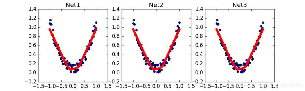
保存和提取参数
import torch
import matplotlib.pyplot as plt

# torch.manual_seed(1)    # reproducible

# fake data
x = torch.unsqueeze(torch.linspace(-1,1,100),dim=1)  # x data (tensor),shape=(100,1) 扩维
y = x.pow(2) + 0.2*torch.rand(x.size())  # noisy y data (tensor),shape=(100,1)

# The code below is deprecated in Pytorch 0.4。Now,autograd directly supports tensors
# x,y = Variable(x,requires_grad=False),Variable(y,requires_grad=False)


def save():
    # save net1
    net1 = torch.nn.Sequential(
        torch.nn.Linear(1,10),
        torch.nn.ReLU(),
        torch.nn.Linear(10,1)
    )
    optimizer = torch.optim.SGD(net1.parameters(),lr=0.5)
    loss_func = torch.nn.MSELoss()

    for t in range(100):
        prediction = net1(x)
        loss = loss_func(prediction,y)
        optimizer.zero_grad()
        loss.backward()
        optimizer.step()

    # plot result
    plt.figure(1,figsize=(10,3))
    plt.subplot(131)
    plt.title('Net1')
    plt.scatter(x.data.numpy(),y.data.numpy())
    plt.plot(x.data.numpy(),prediction.data.numpy(),'r-',lw=5)

    # 2 ways to save the net
    # method 1
    torch.save(net1,'net.pkl')  # save entire net
    # method 2
    torch.save(net1.state_dict(),'net_params.pkl')   # save only the parameters


# 提取神经网络
def restore_net():
    # restore entire net1 to net2
    net2 = torch.load('net.pkl')
    prediction = net2(x)

    # plot result
    plt.subplot(132)
    plt.title('Net2')
    plt.scatter(x.data.numpy(),y.data.numpy())
    plt.plot(x.data.numpy(),prediction.data.numpy(),'r-',lw=5)


def restore_params():
    # restore only the parameters in net1 to net3
    net3 = torch.nn.Sequential(
        torch.nn.Linear(1,10),
        torch.nn.ReLU(),
        torch.nn.Linear(10,1)
    )

    # copy net1's parameters into net3
    net3.load_state_dict(torch.load('net_params.pkl'))
    prediction = net3(x)

    # plot result
    plt.subplot(133)
    plt.title('Net3')
    plt.scatter(x.data.numpy(),y.data.numpy())
    plt.plot(x.data.numpy(),prediction.data.numpy(),'r-',lw=5)
    plt.show()

# save net1
save()

# restore entire net (may slow)
restore_net()

# restore only the net parameters
restore_params()
批训练
Torch 中提供了一种帮你整理你的数据结构的好东西,叫做DataLoader,我们能用它来包装自己的数据,进行批训练。而且批训练可以有很多种途径。
import torch
import torch.utils.data as Data  # 进行批训练的模块

torch.manual_seed(1)    # reproducible

BATCH_SIZE = 5
# BATCH_SIZE = 8

x = torch.linspace(1,10,10)       # this is x data (torch tensor)
y = torch.linspace(10,1,10)       # this is y data (torch tensor)

torch_dataset = Data.TensorDataset(x,y)
loader = Data.DataLoader(
    dataset = torch_dataset,     # torch TensorDataset format
    batch_size = BATCH_SIZE,     # mini batch size
    shuffle = True,              # random shuffle for training  是否要随机打乱数据
    num_workers = 2,             # subprocesses for loading data  多线程 win10可能不兼容
)


def show_batch():
    for epoch in range(3):   # train entire dataset 3 times
        for step,(batch_x,batch_y) in enumerate(loader):  # for each training step
            # train your data...
            print('Epoch: ',epoch,'| Step: ',step,'| batch x: ',
                  batch_x.numpy(),'| batch y: ',batch_y.numpy())


if __name__ == '__main__':
    show_batch()
[外链图片转存失败,源站可能有防盗链机制,建议将图片保存下来直接上传(img-vKssBIvs-1609937985909)(PyTorch-2/batch_train.png)]
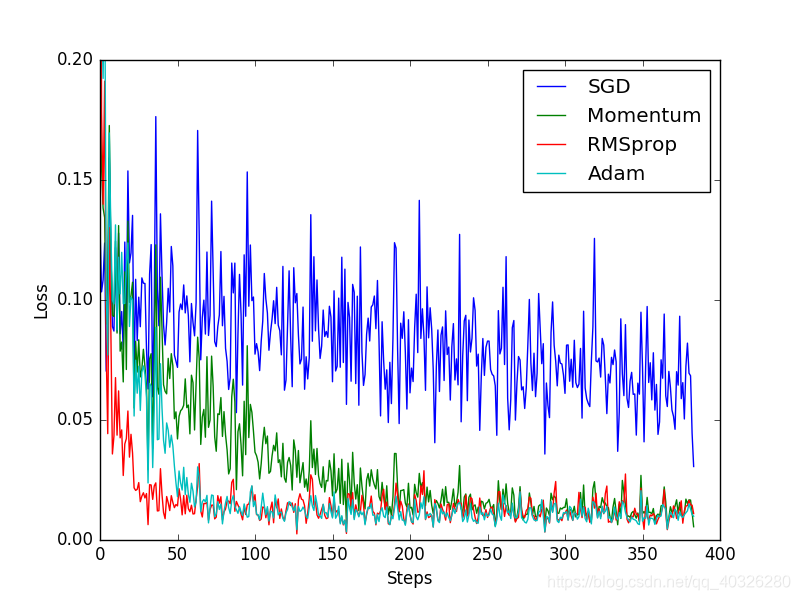
加速神经网络训练
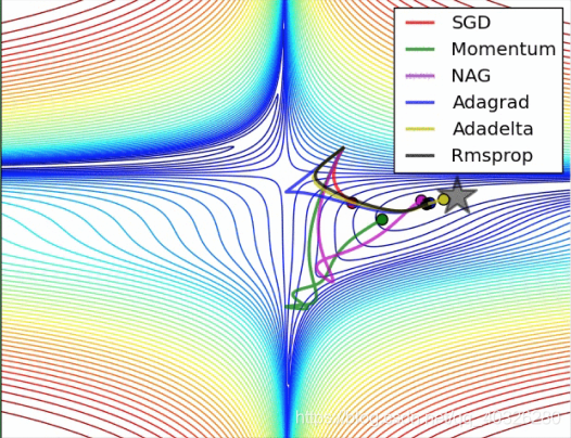
主要区别在权值更新方式
SGD(Stochastic Gradient Descent) 随机梯度下降
W ± − L e a r n i n g R a t e × d x W \pm -LearningRate \times dx W±−LearningRate×dx
Momentum
引入惯性
m = b 1 × m − L e a r n i n g R a t e × d x m = b1 \times m - LearningRate \times dx m=b1×m−LearningRate×dx
W ± m W \pm m W±m
AdaGrad
增加阻力
v ± d x 2 v \pm dx^2 v±dx2
W ± − L e a r n i n g R a t e × d x / r W \pm -LearningRate \times dx /\sqrt{r} W±−LearningRate×dx/r
RMSProp
结合惯性和阻力
v = b 1 × v + ( 1 − b 1 ) × d x 2 v = b1 \times v + (1-b1) \times dx^2 v=b1×v+(1−b1)×dx2
W ± − L e a r n i n g R a t e × d x / v W \pm -LearningRate \times dx/ \sqrt v W±−LearningRate×dx/v
Adam
m = b 1 × m + ( 1 − b 1 ) × d x m = b1 \times m + (1-b1) \times dx m=b1×m+(1−b1)×dx
v = b 2 × v + ( 1 − b 2 ) × d x 2 v = b2 \times v + (1-b2) \times dx^2 v=b2×v+(1−b2)×dx2
W ± − L e a r n i n g R a t e × m / v W \pm -LearningRate \times m / \sqrt{v} W±−LearningRate×m/v
计算m 时有 momentum 下坡的属性,计算 v 时有 adagrad 阻力的属性,然后再更新参数时 把 m 和 V 都考虑进去。实验证明,大多数时候,使用 adam 都能又快又好的达到目标,迅速收敛。
Optimizer优化器
import torch
import torch.utils.data as Data
import torch.nn.functional as F
import matplotlib.pyplot as plt

# torch.manual_seed(1)    # reproducible

# hyper parameters
LR = 0.01
BATCH_SIZE = 32
EPOCH = 12

# fake dataset
x = torch.unsqueeze(torch.linspace(-1,1,1000),dim=1)
y = x.pow(2) + 0.1*torch.normal(torch.zeros(*x.size()))

# plot dataset
plt.scatter(x.numpy(),y.numpy())
plt.show()

# put dateset into torch dataset
torch_dataset = Data.TensorDataset(x,y)  # old version -> Data.TensorDataset(data_tensor=x,target_tensor=y)
loader = Data.DataLoader(dataset=torch_dataset,batch_size=BATCH_SIZE,shuffle=True,num_workers=2,)


# default network
class Net(torch.nn.Module):
    def __init__(self):
        super(Net,self).__init__()
        self.hidden = torch.nn.Linear(1,20)   # hidden layer
        self.predict = torch.nn.Linear(20,1)   # output layer

    def forward(self,x):
        x = F.relu(self.hidden(x))      # activation function for hidden layer
        x = self.predict(x)             # linear output
        return x

if __name__ == '__main__':
    # different nets
    net_SGD         = Net()
    net_Momentum    = Net()
    net_RMSprop     = Net()
    net_Adam        = Net()
    nets = [net_SGD,net_Momentum,net_RMSprop,net_Adam]

    # different optimizers
    opt_SGD         = torch.optim.SGD(net_SGD.parameters(),lr=LR)
    opt_Momentum    = torch.optim.SGD(net_Momentum.parameters(),lr=LR,momentum=0.8)
    opt_RMSprop     = torch.optim.RMSprop(net_RMSprop.parameters(),lr=LR,alpha=0.9)
    opt_Adam        = torch.optim.Adam(net_Adam.parameters(),lr=LR,betas=(0.9,0.99))
    optimizers = [opt_SGD,opt_Momentum,opt_RMSprop,opt_Adam]

    loss_func = torch.nn.MSELoss()
    losses_his = [[],[],[],[]]   # record loss  误差历史记录

    # training
    for epoch in range(EPOCH):
        print('Epoch: ',epoch)
        for step,(b_x,b_y) in enumerate(loader):          # for each training step
            for net,opt,l_his in zip(nets,optimizers,losses_his):
                output = net(b_x)              # get output for every net
                loss = loss_func(output,b_y)  # compute loss for every net
                opt.zero_grad()                # clear gradients for next train
                loss.backward()                # backpropagation,compute gradients
                opt.step()                     # apply gradients
                l_his.append(loss.data.numpy())     # loss recoder

    labels = ['SGD','Momentum','RMSprop','Adam']
    for i,l_his in enumerate(losses_his):
        plt.plot(l_his,label=labels[i])
    plt.legend(loc='best')
    plt.xlabel('Steps')
    plt.ylabel('Loss')
    plt.ylim((0,0.2))
    plt.show()
效果对比:
PyTorch动态神经网络
对比静态动态,我们就得知道谁是静态的。在流行的神经网络模块中,Tensorflow 就是最典型的静态计算模块。下图是一种我在强化学习教程中的 Tensorflow 计算图。也就是说,大部分时候,用 Tensorflow 是先搭建好这样一个计算系统,一旦搭建好了,就不能改动了 (也有例外,比如dynamic_rnn(),但是总体来说他还是运用了一个静态思维),所有的计算都会在这种图中流动,当然很多情况,这样就够了,我们不需要改动什么结构。不动结构当然可以提高效率。但是一旦计算流程不是静态的,计算图要变动。最典型的例子就是 RNN,有时候 RNN 的 time step 不会一样,或者在 training 和 testing 的时候,batch_size 和 time_step 也不一样,这时,Tensorflow 就头疼了,Tensorflow 的人也头疼了。哈哈,如果用一个动态计算图的 Torch,我们就好理解多了,写起来也简单多了。
import torch
from torch import nn
import numpy as np
import matplotlib.pyplot as plt

# torch.manual_seed(1)    # reproducible

# Hyper Parameters
INPUT_SIZE = 1          # rnn input size / image width
LR = 0.02               # learning rate


class RNN(nn.Module):
    def __init__(self):
        super(RNN,self).__init__()

        self.rnn = nn.RNN(
            input_size=1,
            hidden_size=32,    # rnn hidden unit
            num_layers=1,      # number of rnn layer
            batch_first=True,  # input & output will has batch size as 1s dimension。e.g。(batch,time_step,input_size)
        )
        self.out = nn.Linear(32,1)

    def forward(self,x,h_state):
        # x (batch,time_step,input_size)
        # h_state (n_layers,batch,hidden_size)
        # r_out (batch,time_step,output_size)
        r_out,h_state = self.rnn(x,h_state)

        outs = []                                   # this is where you can find torch is dynamic
        for time_step in range(r_out.size(1)):      # calculate output for each time step
            outs.append(self.out(r_out[:,time_step,:]))
        return torch.stack(outs,dim=1),h_state


rnn = RNN()
print(rnn)

optimizer = torch.optim.Adam(rnn.parameters(),lr=LR)   # optimize all cnn parameters
loss_func = nn.MSELoss()                                # the target label is not one-hotted

h_state = None   # for initial hidden state

plt.figure(1,figsize=(12,5))
plt.ion()   # continuously plot

########################  Below is different #########################

################ static time steps ##########
# for step in range(60):
#     start,end = step * np.pi,(step+1)*np.pi   # time steps
#     # use sin predicts cos
#     steps = np.linspace(start,end,10,dtype=np.float32)

################ dynamic time steps #########
step = 0
for i in range(60):
    dynamic_steps = np.random.randint(1,4)  # has random time steps
    start,end = step * np.pi,(step + dynamic_steps) * np.pi  # different time steps length
    step += dynamic_steps

    # use sin predicts cos
    steps = np.linspace(start,end,10 * dynamic_steps,dtype=np.float32)

#######################  Above is different ###########################

    print(len(steps))       # print how many time step feed to RNN

    x_np = np.sin(steps)    # float32 for converting torch FloatTensor
    y_np = np.cos(steps)

    x = torch.from_numpy(x_np[np.newaxis,:,np.newaxis])    # shape (batch,time_step,input_size)
    y = torch.from_numpy(y_np[np.newaxis,:,np.newaxis])

    prediction,h_state = rnn(x,h_state)   # rnn output
    # !! next step is important !!
    h_state = h_state.data        # repack the hidden state,break the connection from last iteration

    loss = loss_func(prediction,y)         # cross entropy loss
    optimizer.zero_grad()                   # clear gradients for this training step
    loss.backward()                         # backpropagation,compute gradients
    optimizer.step()                        # apply gradients

    # plotting
    plt.plot(steps,y_np.flatten(),'r-')
    plt.plot(steps,prediction.data.numpy().flatten(),'b-')
    plt.draw()
    plt.pause(0.05)

plt.ioff()
plt.show()
GPU加速运算
这份 GPU 的代码是依据之前这份CNN的代码修改的。大概修改的地方包括将数据的形式变成 GPU 能读的形式,然后将 CNN 也变成 GPU 能读的形式。做法就是在后面加上 .cuda(),很简单。
"""
View more, visit my tutorial page: https://morvanzhou.github.io/tutorials/
My Youtube Channel: https://www.youtube.com/user/MorvanZhou

Dependencies:
torch: 0.4
torchvision
"""
import torch
import torch.nn as nn
import torch.utils.data as Data
import torchvision

# torch.manual_seed(1)

EPOCH = 1
BATCH_SIZE = 50
LR = 0.001
DOWNLOAD_MNIST = False

train_data = torchvision.datasets.MNIST(root='./mnist/', train=True, transform=torchvision.transforms.ToTensor(), download=DOWNLOAD_MNIST,)
train_loader = Data.DataLoader(dataset=train_data, batch_size=BATCH_SIZE, shuffle=True)

test_data = torchvision.datasets.MNIST(root='./mnist/', train=False)

# !!!!!!!! Change in here !!!!!!!!! #
test_x = torch.unsqueeze(test_data.test_data, dim=1).type(torch.FloatTensor)[:2000].cuda()/255.   # Tensor on GPU
test_y = test_data.test_labels[:2000].cuda()


class CNN(nn.Module):
    def __init__(self):
        super(CNN, self).__init__()
        self.conv1 = nn.Sequential(nn.Conv2d(in_channels=1, out_channels=16, kernel_size=5, stride=1, padding=2,),
                                   nn.ReLU(), nn.MaxPool2d(kernel_size=2),)
        self.conv2 = nn.Sequential(nn.Conv2d(16, 32, 5, 1, 2), nn.ReLU(), nn.MaxPool2d(2),)
        self.out = nn.Linear(32 * 7 * 7, 10)

    def forward(self, x):
        x = self.conv1(x)
        x = self.conv2(x)
        x = x.view(x.size(0), -1)
        output = self.out(x)
        return output

cnn = CNN()

# !!!!!!!! Change in here !!!!!!!!! #
cnn.cuda()      # Moves all model parameters and buffers to the GPU.

optimizer = torch.optim.Adam(cnn.parameters(), lr=LR)
loss_func = nn.CrossEntropyLoss()

for epoch in range(EPOCH):
    for step, (x, y) in enumerate(train_loader):

        # !!!!!!!! Change in here !!!!!!!!! #
        b_x = x.cuda()    # Tensor on GPU
        b_y = y.cuda()    # Tensor on GPU

        output = cnn(b_x)
        loss = loss_func(output, b_y)
        optimizer.zero_grad()
        loss.backward()
        optimizer.step()

        if step % 50 == 0:
            test_output = cnn(test_x)

            # !!!!!!!! Change in here !!!!!!!!! #
            pred_y = torch.max(test_output, 1)[1].cuda().data  # move the computation in GPU

            accuracy = torch.sum(pred_y == test_y).type(torch.FloatTensor) / test_y.size(0)
            print('Epoch: ', epoch, '| train loss: %.4f' % loss.data.cpu().numpy(), '| test accuracy: %.2f' % accuracy)


test_output = cnn(test_x[:10])

# !!!!!!!! Change in here !!!!!!!!! #
pred_y = torch.max(test_output, 1)[1].cuda().data # move the computation in GPU

print(pred_y, 'prediction number')
print(test_y[:10], 'real number')
过拟合(Overfitting)
解决方法:
- 增加训练数据
- 正则化(L1, L2…)
- Dropout regularization
Dropout —— PyTorch实现
"""
View more, visit my tutorial page: https://morvanzhou.github.io/tutorials/
My Youtube Channel: https://www.youtube.com/user/MorvanZhou

Dependencies:
torch: 0.4
matplotlib
"""
import torch
import matplotlib.pyplot as plt

# torch.manual_seed(1)    # reproducible

N_SAMPLES = 20
N_HIDDEN = 300

# training data
x = torch.unsqueeze(torch.linspace(-1, 1, N_SAMPLES), 1)
y = x + 0.3*torch.normal(torch.zeros(N_SAMPLES, 1), torch.ones(N_SAMPLES, 1))

# test data
test_x = torch.unsqueeze(torch.linspace(-1, 1, N_SAMPLES), 1)
test_y = test_x + 0.3*torch.normal(torch.zeros(N_SAMPLES, 1), torch.ones(N_SAMPLES, 1))

# show data
plt.scatter(x.data.numpy(), y.data.numpy(), c='magenta', s=50, alpha=0.5, label='train')
plt.scatter(test_x.data.numpy(), test_y.data.numpy(), c='cyan', s=50, alpha=0.5, label='test')
plt.legend(loc='upper left')
plt.ylim((-2.5, 2.5))
plt.show()

net_overfitting = torch.nn.Sequential(
    torch.nn.Linear(1, N_HIDDEN),
    torch.nn.ReLU(),
    torch.nn.Linear(N_HIDDEN, N_HIDDEN),
    torch.nn.ReLU(),
    torch.nn.Linear(N_HIDDEN, 1),
)

net_dropped = torch.nn.Sequential(
    torch.nn.Linear(1, N_HIDDEN),
    torch.nn.Dropout(0.5),  # drop 50% of the neuron
    torch.nn.ReLU(),
    torch.nn.Linear(N_HIDDEN, N_HIDDEN),
    torch.nn.Dropout(0.5),  # drop 50% of the neuron
    torch.nn.ReLU(),
    torch.nn.Linear(N_HIDDEN, 1),
)

print(net_overfitting)  # net architecture
print(net_dropped)

optimizer_ofit = torch.optim.Adam(net_overfitting.parameters(), lr=0.01)
optimizer_drop = torch.optim.Adam(net_dropped.parameters(), lr=0.01)
loss_func = torch.nn.MSELoss()

plt.ion()   # something about plotting

for t in range(500):
    pred_ofit = net_overfitting(x)
    pred_drop = net_dropped(x)
    loss_ofit = loss_func(pred_ofit, y)
    loss_drop = loss_func(pred_drop, y)

    optimizer_ofit.zero_grad()
    optimizer_drop.zero_grad()
    loss_ofit.backward()
    loss_drop.backward()
    optimizer_ofit.step()
    optimizer_drop.step()

    if t % 10 == 0:
        # change to eval mode in order to fix drop out effect  .eval()切换到预测模型,不屏蔽dropout的神经元
        net_overfitting.eval()
        net_dropped.eval()  # parameters for dropout differ from train mode

        # plotting
        plt.cla()
        test_pred_ofit = net_overfitting(test_x)
        test_pred_drop = net_dropped(test_x)
        plt.scatter(x.data.numpy(), y.data.numpy(), c='magenta', s=50, alpha=0.3, label='train')
        plt.scatter(test_x.data.numpy(), test_y.data.numpy(), c='cyan', s=50, alpha=0.3, label='test')
        plt.plot(test_x.data.numpy(), test_pred_ofit.data.numpy(), 'r-', lw=3, label='overfitting')
        plt.plot(test_x.data.numpy(), test_pred_drop.data.numpy(), 'b--', lw=3, label='dropout(50%)')
        plt.text(0, -1.2, 'overfitting loss=%.4f' % loss_func(test_pred_ofit, test_y).data.numpy(), fontdict={

    'size': 20, 'color':  'red'})
        plt.text(0, -1.5, 'dropout loss=%.4f' % loss_func(test_pred_drop, test_y).data.numpy(), fontdict={

    'size': 20, 'color': 'blue'})
        plt.legend(loc='upper left'); plt.ylim((-2.5, 2.5)); plt.pause(0.1)

        # change back to train mode   切换回训练模式
        net_overfitting.train()
        net_dropped.train()

plt.ioff()
plt.show()
Batch Normalization 批标准化
Batch Normalization,批标准化,和普通的数据标准化类似,是将分散的数据统一的一种做法,也是优化神经网络的一种方法。在之前Normalization 的简介视频中我们一提到,具有统一规格的数据,能让机器学习更容易学习到数据之中的规律。BN操作在全连接层和激励函数之间。
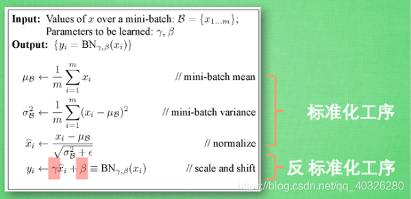
我们引入一些 batch normalization 的公式。这三步就是我们在刚刚一直说的 normalization 工序,但是公式的后面还有一个反向操作,将 normalize 后的数据再扩展和平移。原来这是为了让神经网络自己去学着使用和修改这个扩展参数 gamma,和 平移参数 β,这样神经网络就能自己慢慢琢磨出前面的 normalization 操作到底有没有起到优化的作用,如果没有起到作用,我就使用 gamma 和 belt 来抵消一些 normalization 的操作。
"""
View more, visit my tutorial page: https://morvanzhou.github.io/tutorials/
My Youtube Channel: https://www.youtube.com/user/MorvanZhou

Dependencies:
torch: 0.4
matplotlib
numpy
"""
import torch
from torch import nn
from torch.nn import init
import torch.utils.data as Data
import matplotlib.pyplot as plt
import numpy as np

# torch.manual_seed(1)    # reproducible
# np.random.seed(1)

# Hyper parameters
N_SAMPLES = 2000
BATCH_SIZE = 64
EPOCH = 12
LR = 0.03
N_HIDDEN = 8
ACTIVATION = torch.tanh
B_INIT = -0.2   # use a bad bias constant initializer

# training data
x = np.linspace(-7, 10, N_SAMPLES)[:, np.newaxis]
noise = np.random.normal(0, 2, x.shape)
y = np.square(x) - 5 + noise

# test data
test_x = np.linspace(-7, 10, 200)[:, np.newaxis]
noise = np.random.normal(0, 2, test_x.shape)
test_y = np.square(test_x) - 5 + noise

train_x, train_y = torch.from_numpy(x).float(), torch.from_numpy(y).float()
test_x = torch.from_numpy(test_x).float()
test_y = torch.from_numpy(test_y).float()

train_dataset = Data.TensorDataset(train_x, train_y)
train_loader = Data.DataLoader(dataset=train_dataset, batch_size=BATCH_SIZE, shuffle=True, num_workers=2,)

# show data
plt.scatter(train_x.numpy(), train_y.numpy(), c='#FF9359', s=50, alpha=0.2, label='train')
plt.legend(loc='upper left')


class Net(nn.Module):
    def __init__(self, batch_normalization=False):
        super(Net, self).__init__()
        self.do_bn = batch_normalization
        self.fcs = []
        self.bns = []
        self.bn_input = nn.BatchNorm1d(1, momentum=0.5)   # for input data

        for i in range(N_HIDDEN):               # build hidden layers and BN layers
            input_size = 1 if i == 0 else 10
            fc = nn.Linear(input_size, 10)
            setattr(self, 'fc%i' % i, fc)       # IMPORTANT set layer to the Module
            self._set_init(fc)                  # parameters initialization
            self.fcs.append(fc)
            if self.do_bn:
                bn = nn.BatchNorm1d(10, momentum=0.5)
                setattr(self, 'bn%i' % i, bn)   # IMPORTANT set layer to the Module
                self.bns.append(bn)

        self.predict = nn.Linear(10, 1)         # output layer
        self._set_init(self.predict)            # parameters initialization

    def _set_init(self, layer):
        init.normal_(layer.weight, mean=0., std=.1)
        init.constant_(layer.bias, B_INIT)

    def forward(self, x):
        pre_activation = [x]
        if self.do_bn:
            x = self.bn_input(x)     # input batch normalization
        layer_input = [x]
        for i in range(N_HIDDEN):
            x = self.fcs[i](x)
            pre_activation.append(x)
            if self.do_bn:
                x = self.bns[i](x)   # batch normalization
            x = ACTIVATION(x)
            layer_input.append(x)
        out = self.predict(x)
        return out, layer_input, pre_activation

nets = [Net(batch_normalization=False), Net(batch_normalization=True)]

# print(*nets)    # print net architecture

opts = [torch.optim.Adam(net.parameters(), lr=LR) for net in nets]

loss_func = torch.nn.MSELoss()


def plot_histogram(l_in, l_in_bn, pre_ac, pre_ac_bn):
    for i, (ax_pa, ax_pa_bn, ax, ax_bn) in enumerate(zip(axs[0, :], axs[1, :], axs[2, :], axs[3, :])):
        [a.clear() for a in [ax_pa, ax_pa_bn, ax, ax_bn]]
        if i == 0:
            p_range = (-7, 10);the_range = (-7, 10)
        else:
            p_range = (-4, 4);the_range = (-1, 1)
        ax_pa.set_title('L' + str(i))
        ax_pa.hist(pre_ac[i].data.numpy().ravel(), bins=10, range=p_range, color='#FF9359', alpha=0.5);ax_pa_bn.hist(pre_ac_bn[i].data.numpy().ravel(), bins=10, range=p_range, color='#74BCFF', alpha=0.5)
        ax.hist(l_in[i].data.numpy().ravel(), bins=10, range=the_range, color='#FF9359');ax_bn.hist(l_in_bn[i].data.numpy().ravel(), bins=10, range=the_range, color='#74BCFF')
        for a in [ax_pa, ax, ax_pa_bn, ax_bn]: a.set_yticks(());a.set_xticks(())
        ax_pa_bn.set_xticks(p_range);ax_bn.set_xticks(the_range)
        axs[0, 0].set_ylabel('PreAct');axs[1, 0].set_ylabel('BN PreAct');axs[2, 0].set_ylabel('Act');axs[3, 0].set_ylabel('BN Act')
    plt.pause(0.01)


if __name__ == "__main__":
    f, axs = plt.subplots(4, N_HIDDEN + 1, figsize=(10, 5))
    plt.ion()  # something about plotting
    plt.show()

    # training
    losses = [[], []]  # recode loss for two networks

    for epoch in range(EPOCH):
        print('Epoch: ', epoch)
        layer_inputs, pre_acts = [], []
        for net, l in zip(nets, losses):
            net.eval()              # set eval mode to fix moving_mean and moving_var
            pred, layer_input, pre_act = net(test_x)
            l.append(loss_func(pred, test_y).data.item())
            layer_inputs.append(layer_input)
            pre_acts.append(pre_act)
            net.train()             # free moving_mean and moving_var
        plot_histogram(*layer_inputs, *pre_acts)     # plot histogram

        for step, (b_x, b_y) in enumerate(train_loader):
            for net, opt in zip(nets, opts):     # train for each network
                pred, _, _ = net(b_x)
                loss = loss_func(pred, b_y)
                opt.zero_grad()
                loss.backward()
                opt.step()    # it will also learns the parameters in Batch Normalization

    plt.ioff()

    # plot training loss
    plt.figure(2)
    plt.plot(losses[0], c='#FF9359', lw=3, label='Original')
    plt.plot(losses[1], c='#74BCFF', lw=3, label='Batch Normalization')
    plt.xlabel('step');plt.ylabel('test loss');plt.ylim((0, 2000));plt.legend(loc='best')

    # evaluation
    # set net to eval mode to freeze the parameters in batch normalization layers
    [net.eval() for net in nets]    # set eval mode to fix moving_mean and moving_var
    preds = [net(test_x)[0] for net in nets]
    plt.figure(3)
    plt.plot(test_x.data.numpy(), preds[0].data.numpy(), c='#FF9359', lw=4, label='Original')
    plt.plot(test_x.data.numpy(), preds[1].data.numpy(), c='#74BCFF', lw=4, label='Batch Normalization')
    plt.scatter(test_x.data.numpy(), test_y.data.numpy(), c='r', s=50, alpha=0.2, label='train')
    plt.legend(loc='best')
    plt.show()