[翻译Pytorch教程]NLP从零开始：使用序列到序列网络和注意力机制进行翻译

翻译自官网手册:NLP From Scratch: Translation with a Sequence to Sequence Network and Attention
Author: Sean Robertson
原文github代码
这是NLP从零开始三个教程的第三个。教程中编写了自己的类和函数预处理数据来完成NLP建模任务。希望完成本教程的学习后你可以通过后续的三个教程，继续学习使用torchtext如何完成这些这些任务。

本教程将训练神经网络将法语翻译成英语。

[KEY: > input, = target, < output]

> il est en train de peindre un tableau .
= he is painting a picture .
< he is painting a picture .

> pourquoi ne pas essayer ce vin delicieux ?
= why not try that delicious wine ?
< why not try that delicious wine ?

> elle n est pas poete mais romanciere .
= she is not a poet but a novelist .
< she not not a poet but a novelist .

> vous etes trop maigre .
= you re too skinny .
< you re all alone .

由结果可以看到，取得了不同程度的成功。
简单而强大的思路序列到序列网络sequence
to sequence network使其成为了可能，序列到序列网络中两个循环神经网络共同作用将一个序列转换成另一个序列。一个编码网络将输入序列浓缩成一个向量，一个解码网络将这个向量展开成新的序列。

为了提升模型效果，本文使用了注意力机制（attention
mechanism），其可以让解码器学习关注输入序列的特定范围。

推荐阅读

本教程需要你至少安装了PyTorch、了解Python、了解张量（Tensors）：

• https://pytorch.org/ 安装说明
• Deep Learning with PyTorch: A 60 Minute Blitz 初识PyTorch
• Learning PyTorch with Examples 广泛深入了解
• PyTorch for Former Torch Users 之前使用过Lua Torch

想了解序列到序列网络（Sequence to Sequence networks）及其工作原理：

• Learning Phrase Representations using RNN Encoder-Decoder for
  Statistical Machine Translation
• Sequence to Sequence Learning with Neural
  Networks
• Neural Machine Translation by Jointly Learning to Align and
  Translate
• A Neural Conversational Model

前面教程也可以学习下：

• char_rnn_classification_tutorial
• char_rnn_generation_tutorial

这里的内容分别于编码器和解码器模型比较相似有助于本文理解。

更进一步可以阅读关于这个主题的以下论文：

• Learning Phrase Representations using RNN Encoder-Decoder for
  Statistical Machine Translation
• Sequence to Sequence Learning with Neural
  Networks
• Neural Machine Translation by Jointly Learning to Align and
  Translate
• A Neural Conversational Model

导入所需的库

from __future__ import unicode_literals, print_function, division
from io import open
import unicodedata
import string
import re
import random

import torch
import torch.nn as nn
from torch import optim
import torch.nn.functional as F

device = torch.device("cuda" if torch.cuda.is_available() else "cpu")

加载数据文件（Loading data files）

这个工程的数据是一组几千对英语到法语的翻译对组成。

开放数据集交流平台（Open Data Stack Exchange）上的这个问题将我引到开放翻译网站 https://tatoeba.org/ ，可以从网站下载地址 https://tatoeba.org/eng/downloads 下载数据，更方便的是，有人将语言对分割到独立文本文件中，地址：https://www.manythings.org/anki/

英语-法语对数据太大不能保存在库中，请先在将其下载到 data/eng-fra.txt 目录。这个文件是Tab分割的翻译对列表：

I am cold.    J'ai froid.

注意：
从此处下载数据并解压到当前目录。

与字符级RNN教程中的字母解码器相似，本文将语言中的每个单词表征为独热向量，即除了一个位置（单词索引位置）是1，其余位置全0的向量。与一种语言中可能包含的几十个字母相比，语言有多得多的单词，因此解码向量非常大。本文将对数据进行裁剪，每种语言只使用其中的几千个单词。

每个单词需要有一个独立索引用于后面网络的输入和目标。为了记录这些创建了辅助类Lang ，该类包括单词->索引字典（ word → index，word2index）和索引->单词字典（index → word，index2word），以及每个单词的数量word2count 用于后续过滤掉低频单词。

SOS_token = 0
EOS_token = 1


class Lang:
    def __init__(self, name):
        self.name = name
        self.word2index = {
    
    }
        self.word2count = {
    
    }
        self.index2word = {
    
    0: "SOS", 1: "EOS"}
        self.n_words = 2  # Count SOS and EOS

    def addSentence(self, sentence):
        for word in sentence.split(' '):
            self.addWord(word)

    def addWord(self, word):
        if word not in self.word2index:
            self.word2index[word] = self.n_words
            self.word2count[word] = 1
            self.index2word[self.n_words] = word
            self.n_words += 1
        else:
            self.word2count[word] += 1

文件都是Unicode格式，为了简化将所有Unicode字符转化为ASCII，转化为小写，并过滤掉大部分标点符号。

# 将Unicode字符串转换为简单的ASCII字符，鸣谢 https://stackoverflow.com/a/518232/2809427
def unicodeToAscii(s):
    return ''.join(
        c for c in unicodedata.normalize('NFD', s)
        if unicodedata.category(c) != 'Mn'
    )

# 转小写字母, 裁剪, 移除非字母字符
def normalizeString(s):
    s = unicodeToAscii(s.lower().strip())
    s = re.sub(r"([.!?])", r" \1", s)
    s = re.sub(r"[^a-zA-Z.!?]+", r" ", s)
    return s

读取文件时先将文件分割成行，然后将行分割成句子对。所有的文件都是英语→其他语言格式，如果想将其他语言→英语进行翻译可以使用添加的 reverse标志将句子对进行翻转。

def readLangs(lang1, lang2, reverse=False):
    print("Reading lines...")

    # 读取文件并分割成行
    lines = open('data/%s-%s.txt' % (lang1, lang2), encoding='utf-8').\
        read().strip().split('\n')

    # 将每一行分割成句子对并规范化
    pairs = [[normalizeString(s) for s in l.split('\t')] for l in lines]

    # 如果设置reverse为真则翻转句子对
    # 创建Lang实例
    if reverse:
        pairs = [list(reversed(p)) for p in pairs]
        input_lang = Lang(lang2)
        output_lang = Lang(lang1)
    else:
        input_lang = Lang(lang1)
        output_lang = Lang(lang2)

    return input_lang, output_lang, pairs

由于数据集有很多的样本句子，我们想快速的训练出一些结果，因此将数据集裁剪到相对简短的句子。这里最大长度设置为10个词（包括结束标点），而且过滤剩下格式为 “I am” 和 “He is” 句子。

MAX_LENGTH = 10

eng_prefixes = (
    "i am ", "i m ",
    "he is", "he s ",
    "she is", "she s ",
    "you are", "you re ",
    "we are", "we re ",
    "they are", "they re "
)

#过滤句子对
def filterPair(p):
    return len(p[0].split(' ')) < MAX_LENGTH and \
        len(p[1].split(' ')) < MAX_LENGTH and \
        p[1].startswith(eng_prefixes)

def filterPairs(pairs):
    return [pair for pair in pairs if filterPair(pair)]

预处理数据的全部过程如下：

• 读取文本文件并将其分割到行，将行分割到句子对
• 正规化文本，根据长度和内容过滤句子对
• 创建句子对中句子的单词列表

def prepareData(lang1, lang2, reverse=False):
    input_lang, output_lang, pairs = readLangs(lang1, lang2, reverse)
    print("Read %s sentence pairs" % len(pairs))
    pairs = filterPairs(pairs)
    print("Trimmed to %s sentence pairs" % len(pairs))
    print("Counting words...")
    for pair in pairs:
        input_lang.addSentence(pair[0])
        output_lang.addSentence(pair[1])
    print("Counted words:")
    print(input_lang.name, input_lang.n_words)
    print(output_lang.name, output_lang.n_words)
    return input_lang, output_lang, pairs


input_lang, output_lang, pairs = prepareData('eng', 'fra', True)
print(random.choice(pairs))

Reading lines...
Read 135842 sentence pairs
Trimmed to 10599 sentence pairs
Counting words...
Counted words:
fra 4345
eng 2803
['nous sommes maintenant en phase .', 'we re on the same page now .']

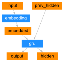
序列到序列模型（The Seq2Seq Model）

循环神经网络是用来处理序列数据的网络结构，其将自身的输出作为下一步的输入。

序列到序列网络、Seq2Seq 网络或编码-解码网络Encoder Decoder
network是由分别被称为编码器和解码器两个RNNs组成的模型。编码器读取输入序列并输出一个单独的向量，解码器读取这个向量并生成输出序列。

不像每个输入对应一个输出的单RNN序列预测，序列到序列（seq2seq）模型将我们从序列长度和顺序中解放出来，这使其成为两种语言翻译的理想选择。

比如句子对 “Je ne suis pas le chat noir” → “I am not the black cat”。输入句子中的大部分单词在输出句子中都可以直接翻译，但是顺序有一些不同，比如：“chat noir” and “black cat”。由于 “ne/pas” 结构输入句子中还多了一个单词。直接根据输入句子单词的顺序处理很难得到正确的翻译。

在seq2seq模型中，编码器创建了一个向量，理想情况下可以将输入句子的含义编码到单个向量（N维句子空间中的一个点）。

编码器（The Encoder）

seq2seq网络的编码器是输入句子每个单词输入时输出一些值的RNN网络。对于每个输入单词编码器输出一个向量和一个隐藏状态，并将隐藏状态用于下一个输入单词。

class EncoderRNN(nn.Module):
    def __init__(self, input_size, hidden_size):
        super(EncoderRNN, self).__init__()
        self.hidden_size = hidden_size

        self.embedding = nn.Embedding(input_size, hidden_size)
        self.gru = nn.GRU(hidden_size, hidden_size)

    def forward(self, input, hidden):
        embedded = self.embedding(input).view(1, 1, -1)
        output = embedded
        output, hidden = self.gru(output, hidden)
        return output, hidden

    def initHidden(self):
        return torch.zeros(1, 1, self.hidden_size, device=device)

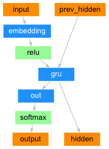
解码器（The Decoder）

解码器接收编码器的输出向量并输出一个序列的单词实现翻译的另一个RNN。

(简单解码器）Simple Decoder

最简单的seq2seq解码器只使用编码器最后的输出进行解码。解码器最后的输出对整个序列的上下文进行了编码，常被称作上下文向量 （context vector）。这个上下文向量被用于初始化解码器的隐藏状态。

每个解码步骤中，传递给解码器一个输入和隐藏状态。初始输入符号是句子的起始字符 <SOS>，第一个隐藏状态是上下文向量（编码器的最终隐藏状态）。

class DecoderRNN(nn.Module):
    def __init__(self, hidden_size, output_size):
        super(DecoderRNN, self).__init__()
        self.hidden_size = hidden_size

        self.embedding = nn.Embedding(output_size, hidden_size)
        self.gru = nn.GRU(hidden_size, hidden_size)
        self.out = nn.Linear(hidden_size, output_size)
        self.softmax = nn.LogSoftmax(dim=1)

    def forward(self, input, hidden):
        output = self.embedding(input).view(1, 1, -1)
        output = F.relu(output)
        output, hidden = self.gru(output, hidden)
        output = self.softmax(self.out(output[0]))
        return output, hidden

    def initHidden(self):
        return torch.zeros(1, 1, self.hidden_size, device=device)

建议你训练并观察这个模型的结果，但是为了缩短篇幅，本文将直接采用最好方案并引入注意力机制（Attention Mechanism）。

注意力解码器（Attention Decoder）

如果只将上下文向量传递给解码器，这单个向量需要承担解码整个句子的任务。

注意力使解码器网络在解码器自己输出的每一步，“聚焦”到解码器输出的不同部分。首先计算一组注意力权重（attention weights）。这将于解码器输出向量相乘来创建一个权重组合。结果（代码中为 attn_applied 变量）包含了输入序列特定部分的信息，有助于帮助解码器选择正确的输出单词。

计算注意力权重是利用另一个前馈层 attn，使用解码器的输入和隐藏状态作为输入。由于训练数据中的句子有各种长度，为了实际创建和训练这一层需要选择最大句子长度（输入长度，对于编码器输出）作为其能处理的长度。最大长度的句子将会利用所有注意力权重，短一点的句子只会使用前面一部分权重。

class AttnDecoderRNN(nn.Module):
    def __init__(self, hidden_size, output_size, dropout_p=0.1, max_length=MAX_LENGTH):
        super(AttnDecoderRNN, self).__init__()
        self.hidden_size = hidden_size
        self.output_size = output_size
        self.dropout_p = dropout_p
        self.max_length = max_length

        self.embedding = nn.Embedding(self.output_size, self.hidden_size)
        self.attn = nn.Linear(self.hidden_size * 2, self.max_length)
        self.attn_combine = nn.Linear(self.hidden_size * 2, self.hidden_size)
        self.dropout = nn.Dropout(self.dropout_p)
        self.gru = nn.GRU(self.hidden_size, self.hidden_size)
        self.out = nn.Linear(self.hidden_size, self.output_size)

    def forward(self, input, hidden, encoder_outputs):
        embedded = self.embedding(input).view(1, 1, -1)
        embedded = self.dropout(embedded)

        attn_weights = F.softmax(
            self.attn(torch.cat((embedded[0], hidden[0]), 1)), dim=1)
        attn_applied = torch.bmm(attn_weights.unsqueeze(0),
                                 encoder_outputs.unsqueeze(0))

        output = torch.cat((embedded[0], attn_applied[0]), 1)
        output = self.attn_combine(output).unsqueeze(0)

        output = F.relu(output)
        output, hidden = self.gru(output, hidden)

        output = F.log_softmax(self.out(output[0]), dim=1)
        return output, hidden, attn_weights

    def initHidden(self):
        return torch.zeros(1, 1, self.hidden_size, device=device)

**注意：**还有一些其他形式的注意力通过使用相对位置方法在长度限制上做工作。可以阅读关于“局部注意力”的Effective Approaches to Attention-based Neural Machine Translation

训练（Training）

准备训练数据（Preparing Training Data）

训练中，对于每个句子对需要输入张量（输入句子中单词的所有）和目标张量（目标句子中单词的索引）。创建了这些张量后，需要在两个序列之后插入终止标记EOS。

def indexesFromSentence(lang, sentence):
    return [lang.word2index[word] for word in sentence.split(' ')]


def tensorFromSentence(lang, sentence):
    indexes = indexesFromSentence(lang, sentence)
    indexes.append(EOS_token)
    return torch.tensor(indexes, dtype=torch.long, device=device).view(-1, 1)


def tensorsFromPair(pair):
    input_tensor = tensorFromSentence(input_lang, pair[0])
    target_tensor = tensorFromSentence(output_lang, pair[1])
    return (input_tensor, target_tensor)

训练模型（Training the Model）

训练中，将输入句子传递给编码器并记录每个输出和最终隐藏状态。输送了 <SOS> 标记作为解码器的第一个输入，编码器的最终隐藏状态作为其第一个隐藏状态。

"Teacher forcing"的概念是使用真实目标输出作为每个下一步输入，而不是使用解码器的预测作为下一步输入。使用"Teacher forcing"导致收敛变快但是当训练网络过度训练，其可能变现的不稳定。

观察teacher-forced网络的输出可以发现，其读取了一致的语法但是输出与正确翻译差距较大，直观来讲解码器学习了如何表征输出语法，如果老师告诉它前几个单词它就能抓住句子的含义，但是它没有很好的学到如何从一开始创建翻译的句子。

由于Pytorch的自动求导的优势，可以随机设置使用和不使用teacher forcing，可以使用teacher_forcing_ratio设定teacher forcing的比例。

teacher_forcing_ratio = 0.5

def train(input_tensor, target_tensor, encoder, decoder, encoder_optimizer, decoder_optimizer, criterion, max_length=MAX_LENGTH):
    encoder_hidden = encoder.initHidden()

    encoder_optimizer.zero_grad()
    decoder_optimizer.zero_grad()

    input_length = input_tensor.size(0)
    target_length = target_tensor.size(0)

    encoder_outputs = torch.zeros(max_length, encoder.hidden_size, device=device)

    loss = 0

    for ei in range(input_length):
        encoder_output, encoder_hidden = encoder(
            input_tensor[ei], encoder_hidden)
        encoder_outputs[ei] = encoder_output[0, 0]

    decoder_input = torch.tensor([[SOS_token]], device=device)

    decoder_hidden = encoder_hidden

    use_teacher_forcing = True if random.random() < teacher_forcing_ratio else False

    if use_teacher_forcing:
        # Teacher forcing: 将目标单词作为下一步输入
        for di in range(target_length):
            decoder_output, decoder_hidden, decoder_attention = decoder(
                decoder_input, decoder_hidden, encoder_outputs)
            loss += criterion(decoder_output, target_tensor[di])
            decoder_input = target_tensor[di]  # Teacher forcing

    else:
        # 关闭 teacher forcing: 使用其自己预测的单词作为下一步输入
        for di in range(target_length):
            decoder_output, decoder_hidden, decoder_attention = decoder(
                decoder_input, decoder_hidden, encoder_outputs)
            topv, topi = decoder_output.topk(1)
            decoder_input = topi.squeeze().detach()  # 将输出解析出来作为输入

            loss += criterion(decoder_output, target_tensor[di])
            if decoder_input.item() == EOS_token:
                break

    loss.backward()

    encoder_optimizer.step()
    decoder_optimizer.step()

    return loss.item() / target_length

这是个可以输出消耗时间、根据当前时间预估的剩余所需时间及进度的百分比的辅助函数。

import time
import math

def asMinutes(s):
    m = math.floor(s / 60)
    s -= m * 60
    return '%dm %ds' % (m, s)

def timeSince(since, percent):
    now = time.time()
    s = now - since
    es = s / (percent)
    rs = es - s
    return '%s (- %s)' % (asMinutes(s), asMinutes(rs))

整个训练过程如下：

• 开启计时器
• 初始化优化器和标准
• 创建训练句子对集合
• 初始化用于绘图的空损失数组

随之，调用train很多次并偶尔输出训练进程（样本的百分比，目前消耗的时间，预估时间）和平均损失。

def trainIters(encoder, decoder, n_iters, print_every=1000, plot_every=100, learning_rate=0.01):
    start = time.time()
    plot_losses = []
    print_loss_total = 0  # 重置每一个 print_every
    plot_loss_total = 0  # 重置每一个 plot_every

    encoder_optimizer = optim.SGD(encoder.parameters(), lr=learning_rate)
    decoder_optimizer = optim.SGD(decoder.parameters(), lr=learning_rate)
    training_pairs = [tensorsFromPair(random.choice(pairs))
                      for i in range(n_iters)]
    criterion = nn.NLLLoss()

    for iter in range(1, n_iters + 1):
        training_pair = training_pairs[iter - 1]
        input_tensor = training_pair[0]
        target_tensor = training_pair[1]

        loss = train(input_tensor, target_tensor, encoder,
                     decoder, encoder_optimizer, decoder_optimizer, criterion)
        print_loss_total += loss
        plot_loss_total += loss

        if iter % print_every == 0:
            print_loss_avg = print_loss_total / print_every
            print_loss_total = 0
            print('%s (%d %d%%) %.4f' % (timeSince(start, iter / n_iters),
                                         iter, iter / n_iters * 100, print_loss_avg))

        if iter % plot_every == 0:
            plot_loss_avg = plot_loss_total / plot_every
            plot_losses.append(plot_loss_avg)
            plot_loss_total = 0

    showPlot(plot_losses)

绘制结果（Plotting results）

调用matplotlib，使用训练时保存的损失值数组plot_losses 绘制图像。

import matplotlib.pyplot as plt
plt.switch_backend('agg')
import matplotlib.ticker as ticker
import numpy as np


def showPlot(points):
    plt.figure()
    fig, ax = plt.subplots()
    # 这个定位器将钩子放置到定期间隔
    loc = ticker.MultipleLocator(base=0.2)
    ax.yaxis.set_major_locator(loc)
    plt.plot(points)

评估（Evaluation）

评估大部分与训练相同，但是这里没有目标输出，因此只要简单的将解码器每一步预测的输出作为输入传递给自己。每次其预测一个单词就将其插入到输出字符串，如果其预测时EOS标记则终止循环。也保存了解码器的注意力输出用于后面展示。

def evaluate(encoder, decoder, sentence, max_length=MAX_LENGTH):
    with torch.no_grad():
        input_tensor = tensorFromSentence(input_lang, sentence)
        input_length = input_tensor.size()[0]
        encoder_hidden = encoder.initHidden()

        encoder_outputs = torch.zeros(max_length, encoder.hidden_size, device=device)

        for ei in range(input_length):
            encoder_output, encoder_hidden = encoder(input_tensor[ei],
                                                     encoder_hidden)
            encoder_outputs[ei] += encoder_output[0, 0]

        decoder_input = torch.tensor([[SOS_token]], device=device)  # SOS

        decoder_hidden = encoder_hidden

        decoded_words = []
        decoder_attentions = torch.zeros(max_length, max_length)

        for di in range(max_length):
            decoder_output, decoder_hidden, decoder_attention = decoder(
                decoder_input, decoder_hidden, encoder_outputs)
            decoder_attentions[di] = decoder_attention.data
            topv, topi = decoder_output.data.topk(1)
            if topi.item() == EOS_token:
                decoded_words.append('<EOS>')
                break
            else:
                decoded_words.append(output_lang.index2word[topi.item()])

            decoder_input = topi.squeeze().detach()

        return decoded_words, decoder_attentions[:di + 1]

可以评估在训练集中随机选取的句子并打印出输入、目标和输出来进行主观上的质量评价。

def evaluateRandomly(encoder, decoder, n=10):
    for i in range(n):
        pair = random.choice(pairs)
        print('>', pair[0])
        print('=', pair[1])
        output_words, attentions = evaluate(encoder, decoder, pair[0])
        output_sentence = ' '.join(output_words)
        print('<', output_sentence)
        print('')

训练和评估（Training and Evaluating）

准备好这些辅助函数（看起来是多余的工作，但是其使多次运行实验变得简单）可以真正初始化网络并开始训练。

注意输入句子已经被高度过滤了。对于这个较小的数据集可以使用相对较小256个隐藏节点和单GRU层的网络。在MacBook CPU上经过40分钟的训练，可以得到比较合理的结果。

注意：
如果运行这个笔记，你可以训练、中断kernel、评估、中断后过段时间继续训练。注释掉给编码器和解码器初始化的代码，并再次运行trainIters。

hidden_size = 256
encoder1 = EncoderRNN(input_lang.n_words, hidden_size).to(device)
attn_decoder1 = AttnDecoderRNN(hidden_size, output_lang.n_words, dropout_p=0.1).to(device)

trainIters(encoder1, attn_decoder1, 75000, print_every=5000)
# trainIters(encoder1, attn_decoder1, 5000, print_every=5000)

输出：

2m 53s (- 40m 28s) (5000 6%) 2.8583
5m 17s (- 34m 25s) (10000 13%) 2.2744
8m 25s (- 33m 40s) (15000 20%) 1.9588
11m 18s (- 31m 4s) (20000 26%) 1.7172
14m 25s (- 28m 51s) (25000 33%) 1.4879
17m 33s (- 26m 19s) (30000 40%) 1.3636
20m 40s (- 23m 37s) (35000 46%) 1.1947
23m 40s (- 20m 43s) (40000 53%) 1.0752
26m 48s (- 17m 52s) (45000 60%) 0.9918
29m 13s (- 14m 36s) (50000 66%) 0.8743
31m 54s (- 11m 36s) (55000 73%) 0.8082
35m 3s (- 8m 45s) (60000 80%) 0.7371
37m 23s (- 5m 45s) (65000 86%) 0.6314
39m 57s (- 2m 51s) (70000 93%) 0.6065
43m 5s (- 0m 0s) (75000 100%) 0.5481

evaluateRandomly(encoder1, attn_decoder1)

输出：

> je ne suis pas du tout romantique .
= i am not romantic at all .
< i am not at at all . <EOS>

> ils ne sont pas du tout interesses .
= they are not at all interested .
< they are not at all interested . <EOS>

> vous etes paresseux .
= you re lazy .
< you re lazy . <EOS>

> nous ne sommes pas en train d evacuer .
= we re not evacuating .
< we re not smiling . <EOS>

> nous avons tous deux tort .
= we re both wrong .
< we re both wrong . <EOS>

> vous etes arrogants .
= you re arrogant .
< you re aggressive . <EOS>

> je suis fatigue d ecouter tom .
= i am tired of listening to tom .
< i m tired of listening to tom . <EOS>

> je suis fort impressionnee .
= i m very impressed .
< i m definitely impressed . <EOS>

> vous n avez plus d excuses .
= you re out of excuses .
< you re out of excuses . <EOS>

> elle a loupe le coche .
= she s missed the boat .
< she s missed the boat . <EOS>

可视化注意力（Visualizing Attention）

注意力机制一个很有用的特性是其高可解释的输出。由于它是用于权重输入序列的特定编码器输出，可以画图查看在每个时间步网络的注意力在哪。

可以简单的运行 plt.matshow(attentions) 查看展示成矩阵的注意力输出，其中列是输入步数、行是输出步数。

output_words, attentions = evaluate(
    encoder1, attn_decoder1, "je suis trop froid .")
plt.matshow(attentions.numpy())

为了更好的观察实验，为图像添加了坐标和标签。

def showAttention(input_sentence, output_words, attentions):
    # 设置图片颜色条
    fig = plt.figure()
    ax = fig.add_subplot(111)
    cax = ax.matshow(attentions.numpy(), cmap='bone')
    fig.colorbar(cax)

    # 设置坐标轴
    ax.set_xticklabels([''] + input_sentence.split(' ') +
                       ['<EOS>'], rotation=90)
    ax.set_yticklabels([''] + output_words)

    # 展示每个标记的标签
    ax.xaxis.set_major_locator(ticker.MultipleLocator(1))
    ax.yaxis.set_major_locator(ticker.MultipleLocator(1))

    plt.show()

def evaluateAndShowAttention(input_sentence):
    output_words, attentions = evaluate(
        encoder1, attn_decoder1, input_sentence)
    print('input =', input_sentence)
    print('output =', ' '.join(output_words))
    showAttention(input_sentence, output_words, attentions)

evaluateAndShowAttention("elle a cinq ans de moins que moi .")

evaluateAndShowAttention("elle est trop petit .")

evaluateAndShowAttention("je ne crains pas de mourir .")

evaluateAndShowAttention("c est un jeune directeur plein de talent .")

输出：

input = elle a cinq ans de moins que moi .
output = she s five years younger than i am . <EOS>

input = elle est trop petit .
output = she is too short . <EOS>

input = je ne crains pas de mourir .
output = i m not scared of dying . <EOS>

input = c est un jeune directeur plein de talent .
output = he is a great young man . <EOS>

练习（Exercises）

• 尝试不同的数据集
  • 使用其他语言对
  • 人机交互：Human → Machine (e.g. IOT commands)
  • 聊天→回答：Chat → Response
  • 问答：Question → Answer
• 使用预训练的词嵌入如word2vec或GloVe代替词嵌入
• 尝试更多层、更多隐藏单元、更多句子，并对比训练时间和结果。
• 如果使用句子对是相同句子(I am test \t I am test)的翻译文件，可以当作是自编码器，尝试：
  • 训练一个自编码器
  • 只保存编码器网络
  • 从上步保存的编码器训练一个新的解码器