PCL：点云特征描述子3D_object_recognition_(descriptors)

现在是学习点云处理最有趣应用之一的基础知识的时候了:3D对象识别。与2D识别类似，该技术依赖于在云中找到好的关键点(特征点)，并将它们与之前保存的一组关键点进行匹配。但是3D比2D有几个优势:也就是说，我们能够相对于传感器精确地估计物体的确切位置和方向。此外，3D对象识别往往对于杂乱的环境有更强大的鲁棒性(比如在比较拥挤的场景，前面的物体会遮挡住在后边背景中物体)。最后，掌握物体形状的信息将有助于避免碰撞或抓取操作。

在第一个教程中，我们将了解什么是描述符，PCL中有多少类型可用，以及如何计算它们。

1、概述

3D对象识别的基础是在两个不同的云之间找到一组对应关系，其中一个包含我们要寻找的对象。为此，我们需要一种以明确的方式比较点的方法。到现在为止，我们已经使用了存储XYZ坐标，RGB颜色的点，但是这些属性都不够独特。在两次连续扫描中，尽管属于不同表面，但两个点仍可以共享相同的坐标，and using the color information takes us back to 2D recognition, will all the lightning related problems。

feature（特征）讨论见文章：https://blog.csdn.net/m0_37957160/article/details/108405087

在之前的教程中，在介绍法线之前我们讨论了特征（feature）。法线是特征的一个例子，因为它们编码关于点附近的信息。也就是说，计算时要考虑到相邻的点，这样我们就可以了解周围的表面是怎样的了。但这还不够。一个特征要想是最佳的，它必须满足以下条件：

1.It must be robust to transformations: 像平移和旋转这样的刚体变换(并不改变点之间距离的变换)一定不会影响特征。Even if we play with the cloud a bit beforehand, there should be no difference。

2.It must be robust to noise:产生的噪声的测量误差不应对特征估计造成太大影响。（对噪声鲁棒性）

3.It must be resolution invariant: 如果进行不同密度的采样(如执行下降采样)，结果必须相同或相似。

这就是描述符的作用。点的特征越复杂(和精确)，他们就会编码大量关于周围几何图形的信息。其目的是在多个点云之间明确地识别一个点，不管噪声、分辨率或变换。另外，描述符获取一些关于它们所属对象的额外数据，比如视点(可以让我们检索姿态)。

Finding correspondences between point features of two clouds (image from http://pointclouds.org/

PCL中实现了许多3D描述符。每一个描述符都有它自己的方法来计算一个点的唯一值。例如，某些方法会使用该点及其相邻点的法线角度之间的差异。其他方法则使用两点之间的距离。因此，对于一定的标准目标，一些方法可能是好的也可能是坏的。一个给定的描述符可能是尺度不变的，而另一个描述符可能对于遮挡和物体局部视图是更好的。选择哪种描述符取决于你要做什么。

关于直方图的介绍见链接：

计算完必要的值（the necessary values）之后，执行附加步骤以减小描述符的大小：并将结果合并到直方图中。为此，将构成描述符的每个变量的值范围划分为n个细分，并计算每个变量中出现的次数。试着想象一个计算单个变量的描述符，它的范围从1到100，我们选择为它创建10个bins(容器)，因此第一个bin将收集1到10之间的所有匹配项，第二个bin将收集11到20之间的所有匹配项，依此类推。我们看一下第一个点-邻居对的变量值，它是27，所以我们将第三个bin的值（也就是20到30的bin划分）增加1。我们一直这样做，直到获得该关键点的最终直方图。必须根据该变量的描述性来仔细选择bin的大小（变量不必共享相同数量的bins，并且bins的大小也不必相同；例如，如果前一个示例中的大多数值都在50-100范围内，那么在该范围内使用更多较小大小的容器将是明智的)。

描述符可分为两大类:全局描述符和局部描述符。计算和使用每一个(比如识别管道)的过程是不同的，因此本文将在各自的部分中进行解释。

Tutorials:

How 3D Features work in PCL：链接如下：博客翻译链接如下
Overview and Comparison of Features：链接如下：https://github.com/PointCloudLibrary/pcl/wiki/Overview-and-Comparison-of-Features 博客翻译链接如下：
How does a good feature look like?链接如下：博客翻译链接如下

Publication:

Point Cloud Library: Three-Dimensional Object Recognition and 6 DoF Pose Estimation (Aitor Aldoma et al., 2012)

下表将告诉你PCL中有多少描述符，以及它们的一些特性:

† Values marked with an asterisk (*) indicate that the descriptor's size depends on some parameter(s), and the one given is for the default values.

†† Descriptors without their own custom PointType use the generic "pcl::Histogram<>" type. See Saving and loading(链接：http://robotica.unileon.es/index.php/PCL/OpenNI_tutorial_4:_3D_object_recognition_(descriptors)#Saving_and_loading)

Optionally, you can download a document with a less simple version of the table. Page format is A4, landscape:

Local descriptors

局部描述符是为我们作为输入的单个点计算的。他们对物体是什么样子没有概念（不知道物体是什么），他们只是描述了这个点周围的局部几何是怎么样的。通常，您的任务是选择需要为哪些点计算描述符:即关键点。在大多数情况下，您可以通过执行下采样并选择所有剩余点来摆脱困境，但是可以使用关键点检测器，例如用于NARF（见下方）或ISS的检测器（见链接：http://robotica.unileon.es/index.php/PCL/OpenNI_tutorial_5:_3D_object_recognition_(pipeline)#ISS）。

Local descriptors are used for object recognition and registration（见链接：http://robotica.unileon.es/index.php/PCL/OpenNI_tutorial_3:_Cloud_processing_(advanced)#Registration）. Now we will see which ones are implemented into PCL.

1）PFH

PFH代表点特征直方图。它是PCL提供的最重要的描述符之一，也是其他(如FPFH)的基础。PFH试图通过分析该点附近法线方向的差异来捕获该点周围的几何信息(正因为如此，不精确的法线估计可能产生低质量的描述符)。

首先，该算法将附近的所有点配对（不仅将选定的关键点与其邻居配对，而且还将邻居与其自身配对）(First, the algorithm pairs all points in the vicinity (not just the chosen keypoint with its neighbors, but also the neighbors with themselves).)。然后，对于每一对，根据其法线计算固定坐标系。在此框架下，法线之间的差异可以用3个角度变量进行编码。保存这些变量以及点之间的欧几里得距离，然后在计算所有点对时将它们合并到直方图中。 The final descriptor is the concatenation of the histograms of each variable (4 in total). （总共4个）。

-----自己个人理解-----

点特征的描述子一般是基于点坐标、法向量、曲率来描述某个点周围的几何特征。用点特征描述子不能提供特征之间的关系，减少了全局特征信息。因此诞生了一直基于直方图的特征描述子：PFH--point feature histogram（点特征直方图）。

2.PFH的原理

PFH通过参数化查询点和紧邻点之间的空间差异，形成了一个多维直方图对点的近邻进行几何描述，直方图提供的信息对于点云具有平移旋转不变性，对采样密度和噪声点具有稳健性。PFH是基于点与其邻近之间的关系以及它们的估计法线，也即是它考虑估计法线之间的相互关系，来描述几何特征。

为了计算两个点（ ps is deﬁned as the source point and pt as the target point）及其相关法线之间的偏差，在其中一个点上定义了一个固定坐标系。

使用上图的uvw坐标系，法线ns，nt之间的偏差可以用一组角度表示

d是两点之间的欧氏距离，，利用α,φ,θ,d，四个元素可以构成PFH描述子。

问题来了，PFH翻译成点特征直方图，四个元素和直方图有什么关系？

首先计算查询点Pq近邻内的对应的所有四个元素，如图所示，表示的是一个查询点(Pq) 的PFH计算的影响区域，Pq 用红色标注并放在圆球的中间位置，半径为r， (Pq)的所有k邻元素（即与点Pq的距离小于半径r的所有点）全部互相连接在一个网络中。最终的PFH描述子通过计算邻域内所有两点之间关系而得到的直方图，因此存在一个O(k) 的计算复杂性。

为了创建最终的直方图，将所有四元素组以统计的方式放入一个直方图中，这个过程首先把每个特征值范围划分为b个子区间，并统计落在每个子区间的点数量，前三个元素均是角度，都和法向量有关系，可以将三个元素标准化并放到同一个区间内。

横坐标表示角度，纵坐标表示区间内点云的数量。

3.FPFH的由来

具有n个点的点云p的点特征直方图的理论计算复杂度为o（nk^2），其中k是点云p中每个点p的邻近数。在密集点邻域中计算点特征柱状图可以表示映射框架中的主要瓶颈之一。本节提出了PFH公式的简单化，称为快速点特征直方图（FPFH:fast point feature histograms），它将算法的计算复杂度降低到O（NK），同时仍然保留了PFH的大部分判别能力。

4.FPFH的原理

step1，只计算每个查询点Pq和它邻域点之间的三个特征元素（参考PFH），在这里不同于PFH：PFH是计算邻域点所有组合的特征元素，而这一步只计算查询点和近邻点之间的特征元素。如下图，第一个图是PFH计算特征过程，即邻域点所有组合的特征值（图中所有连线，包括但不限于Pq和Pk之间的连线），第二个图是step1中计算内容，只需要计算Pq（查询点）和紧邻点（图2中红线部分）之间的特征元素。可以看出降低了复杂度我们称之为SPFH（simple point feature histograms）。

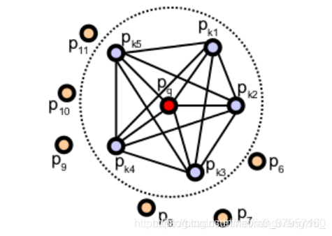
(看清楚两个图的区别，一个是PFH所有点之间的关系，一个是FPFH只考虑当前关键点与其相邻节点之间的直接连接，删除相邻节点之间的附加连接。)

step2，重新确定k近邻域，为了确定查询点Pq的近邻点Pk的SPFH值、查询点Pq和近邻的距离以及k的数值（一般使用半径kdtree搜索，只能确定某半径范围内的近邻点，不能确定具体的查询点与近邻的距离、k数值----PS:应该是这样，不过重新确定k近邻主要还是计算查询点Pq的近邻点Pk的SPFH值），则

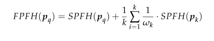
Wk权重，一般为距离。

这里的FPFH是由查询点 $p_{q}$ 的简化特征直方图SPFH（ $p_{q}$ ）加上周边K邻域内的各个邻域点的SPFH( $p_{k}$ )的加权和两部分构成，SPFH（ $p_{q}$ )或SPFH(pk)的每个区间内的值都是整数，且区间内的值加起来等于邻域内的邻域点数。但是每个区间经过后半部的加权之后，使得最终的FPFH(pq)的每个区间变成了小数。

5.二者区别和联系

（1）FPFH没有对近邻点所有组合进行计算可能漏掉一些重要点对

（2）PFH特征模型是对查询点周围精确的邻域半径内，而FPFH还包括半径r范围以外的额外点对（不过在2r内，这是由于计算SPFH(Pk)导致的）

（3）FPFH降低了复杂度，可以在实时场景中使用

（4）因为重新计算权重，所以FPFH结合SPFH值，重新获取重要的紧邻点对几何信息

（5）在FPFH中，通过分解三元组（三个角特征）简化了合成的直方图，即简单地创建b个相关的的特征直方图，每个特征维数（dimension）对应一个直方图（bin），并将它们连接在一起。pcl默认，in PFH assume the number of quantum bins (i.e. subdivision intervals in a feature’s value range),bins（b）=5即子区间数量（为什么默认5不知道），三个角特征元素，5^3=125,（至于为什么5的3次方不知道？？？）也就是一个查询点就有125个子区间，PFHSignature125的由来。这样有一个问题：对于点云特别是稀疏点云来说，很多区间存在0值，即直方图上存在冗余空间。因此，在FPFH中，通过分解三元组（三个角特征）简化了合成的直方图，即简单地创建b个不相关的的特征直方图，每个特征维数（dimension）对应一个直方图（bin），并将它们连接在一起。pcl默认FPFH的b=11，3*11=33，也就是FPFHSignature33的由来。

参考文献：RUSU博士论文，以及RUSU发表的会议论文Fast Point Feature Histograms (FPFH) for 3D Registration

参考链接：http://www.pclcn.org/study/shownews.php?id=101

-------个人理解结束，接着翻译理解------

计算描述符在PCL是非常容易的，PFH也不例外:

#include <pcl/io/pcd_io.h>
#include <pcl/features/normal_3d.h>
#include <pcl/features/pfh.h>

int
main(int argc, char** argv)
{
	// Object for storing the point cloud.//储存点云对象
	pcl::PointCloud<pcl::PointXYZ>::Ptr cloud(new pcl::PointCloud<pcl::PointXYZ>);
	// Object for storing the normals.//储存法线对象
	pcl::PointCloud<pcl::Normal>::Ptr normals(new pcl::PointCloud<pcl::Normal>);
	// Object for storing the PFH descriptors for each point.建立用于存储每个点的PFH描述符的对象。
	pcl::PointCloud<pcl::PFHSignature125>::Ptr descriptors(new pcl::PointCloud<pcl::PFHSignature125>());

	// Read a PCD file from disk.//读取
	if (pcl::io::loadPCDFile<pcl::PointXYZ>(argv[1], *cloud) != 0)
	{
		return -1;
	}

	// Note: you would usually perform downsampling now. It has been omitted here
	// for simplicity, but be aware that computation can take a long time.
        （注意:您通常现在执行向下采样。这里省略了，为了简单起见，但是要注意计算可能会花费很长时间。）

	// Estimate the normals.//计算发现
	pcl::NormalEstimation<pcl::PointXYZ, pcl::Normal> normalEstimation;
	normalEstimation.setInputCloud(cloud);
	normalEstimation.setRadiusSearch(0.03);
	pcl::search::KdTree<pcl::PointXYZ>::Ptr kdtree(new pcl::search::KdTree<pcl::PointXYZ>);
	normalEstimation.setSearchMethod(kdtree);
	normalEstimation.compute(*normals);

	// PFH estimation object.
	pcl::PFHEstimation<pcl::PointXYZ, pcl::Normal, pcl::PFHSignature125> pfh;
	pfh.setInputCloud(cloud);
	pfh.setInputNormals(normals);
	pfh.setSearchMethod(kdtree);
	// Search radius, to look for neighbors. Note: the value given here has to be
	// larger than the radius used to estimate the normals.
	pfh.setRadiusSearch(0.05);

	pfh.compute(*descriptors);
}

As you can see, PCL uses the "PFHSignature125" type to save the descriptor to. This means that the descriptor's size is 125 (the dimensionality of the feature vector). Dividing a feature in D dimensional space in B divisions requires a total of $B^{D}$ bins. The original proposal makes use of the distance between the points, but the implementation of PCL does not, as it was not considered discriminative enough (specially in 2.5D scans, where the distance between points increases the further away from the sensor). Hence, the remaining features (with one dimension each) can be divided in 5 divisions, resulting in a 125-dimensional ( $5^{3}$ ) vector.

The final object that stores the computed descriptors can be handled like a normal cloud (even saved to, or read from, disk), and it has the same number of "points" than the original one. The "PFHSignature125" object at position 0, for example, stores the PFH descriptor for the "PointXYZ" point at the same position in the cloud.

Input: Points, Normals, Search method, Radius
Output: PFH descriptors
Tutorial: Point Feature Histograms (PFH) descriptors
Publications:
- Persistent Point Feature Histograms for 3D Point Clouds (Radu Bogdan Rusu et al., 2008)
- Semantic 3D Object Maps for Everyday Manipulation in Human Living Environments (Radu Bogdan Rusu, 2009, section 4.4, page 50)
API: pcl::PFHEstimation(官网API函数)
Download（这个链接没有）

2）PFH

PFH给出了准确的结果，但它有一个缺点:它的计算成本太高，无法实时执行。对于考虑了n个关键点和k个邻居的云，它的复杂度为 $O(nk^{2})$ 。因此，一个派生描述符被创建，名为FPFH (Fast Point Feature Histogram)。

FPFH只考虑当前关键点与其相邻节点之间的直接连接，删除相邻节点之间的附加连接。这将复杂性降低到O(nk)。因此，得到的直方图称为SPFH(简化点特征直方图)。参考系和角变量一如既往地计算。

FPFH只考虑当前关键点与其相邻节点之间的直接连接，删除相邻节点之间的附加连接。这将复杂性降低到O(nk)。因此，得到的直方图称为SPFH(简化点特征直方图)。参考系和角变量一如既往地计算。（The reference frame and the angular variables are computed as always. ）

为了解决这些额外连接的丢失，在计算完所有直方图之后，需要执行一个附加步骤：将点的邻居的SPFH与自己的邻居的SPFH“合并”，并根据距离加权。这样的效果是可以给出远至所用半径2倍的点的点表面信息。最后，将3个直方图（不使用距离）连接起来组成最终的描述符。

(To account for the loss of these extra connections, an additional step takes place after all histograms have been computed: the SPFHs of a point's neighbors are "merged" with its own, weighted according to the distance. This has the effect of giving a point surface information of points as far away as 2 times the radius used. Finally, the 3 histograms (distance is not used) are concatenated to compose the final descriptor. )

#include <pcl/io/pcd_io.h>
#include <pcl/features/normal_3d.h>
#include <pcl/features/fpfh.h>

int
main(int argc, char** argv)
{
	// Object for storing the point cloud.
	pcl::PointCloud<pcl::PointXYZ>::Ptr cloud(new pcl::PointCloud<pcl::PointXYZ>);
	// Object for storing the normals.
	pcl::PointCloud<pcl::Normal>::Ptr normals(new pcl::PointCloud<pcl::Normal>);
	// Object for storing the FPFH descriptors for each point.
	pcl::PointCloud<pcl::FPFHSignature33>::Ptr descriptors(new pcl::PointCloud<pcl::FPFHSignature33>());

	// Read a PCD file from disk.
	if (pcl::io::loadPCDFile<pcl::PointXYZ>(argv[1], *cloud) != 0)
	{
		return -1;
	}

	// Note: you would usually perform downsampling now. It has been omitted here
	// for simplicity, but be aware that computation can take a long time.

	// Estimate the normals.
	pcl::NormalEstimation<pcl::PointXYZ, pcl::Normal> normalEstimation;
	normalEstimation.setInputCloud(cloud);
	normalEstimation.setRadiusSearch(0.03);
	pcl::search::KdTree<pcl::PointXYZ>::Ptr kdtree(new pcl::search::KdTree<pcl::PointXYZ>);
	normalEstimation.setSearchMethod(kdtree);
	normalEstimation.compute(*normals);

	// FPFH estimation object.
	pcl::FPFHEstimation<pcl::PointXYZ, pcl::Normal, pcl::FPFHSignature33> fpfh;
	fpfh.setInputCloud(cloud);
	fpfh.setInputNormals(normals);
	fpfh.setSearchMethod(kdtree);
	// Search radius, to look for neighbors. Note: the value given here has to be
	// larger than the radius used to estimate the normals.
	fpfh.setRadiusSearch(0.05);

	fpfh.compute(*descriptors);
}

类“ FPFHEstimationOMP”中提供了利用多线程优化（带有OpenMP API）的FPFH估计的其他实现。其接口与标准未优化的实现相同。使用它会大大提高多核系统的性能，这意味着更快的计算时间。请记住要改为包含标题“ fpfh_omp.h”。

Input: Points, Normals, Search method, Radius
Output: FPFH descriptors
Tutorial: Fast Point Feature Histograms (FPFH) descriptors
Publications:
- Fast Point Feature Histograms (FPFH) for 3D Registration (Radu Bogdan Rusu et al., 2009)
- Semantic 3D Object Maps for Everyday Manipulation in Human Living Environments (Radu Bogdan Rusu, 2009, section 4.5, page 57)
API:
- pcl::FPFHEstimation
- pcl::FPFHEstimationOMP
Download

3)RSD （后边的除了VFH自己会用到，详细理解，其他的都只是粘贴英文）

先翻译未深入理解，用到再看

The Radius-Based Surface Descriptor encodes the radial relationship of the point and its neighborhood. For every pair of the keypoint with a neighbor, the algorithm computes the distance between them, and the difference between their normals. Then, by assuming that both points lie on the surface of a sphere, said sphere is found by fitting not only the points, but also the normals (otherwise, there would be infinite possible spheres). Finally, from all the point-neighbor spheres, only the ones with the maximum and minimum radii are kept and saved to the descriptor of that point.

As you may have deduced already, when two points lie on a flat surface, the sphere radius will be infinite. If, on the other hand, they lie on the curved face of a cylinder, the radius will be more or less the same as that of the cylinder. This allows us to tell objects apart with RSD. The algorithm takes a parameter that sets the maximum radius at which the points will be considered to be part of a plane.

基于半径的表面描述符对点及其邻域的径向关系进行编码。对于与邻居的每对关键点，算法都会计算它们之间的距离以及它们的法线之间的差。然后，通过假设两个点都位于球体的表面上，不仅可以拟合这些点，还可以拟合法线来找到该球体（否则，将存在无限可能的球体）。最后，在所有点相邻球体中，只有半径最大和最小的球体才会保留并保存到该点的描述符中。
正如您可能已经推论的那样，当两个点位于一个平面上时，球体半径将是无限的。另一方面，如果它们位于圆柱体的曲面上，则半径将与圆柱体的半径大致相同。这使我们可以区分对象与RSD。该算法采用一个参数，该参数设置将点视为平面一部分的最大半径。

这是编译RSD描述符的代码:

#include <pcl/io/pcd_io.h>
#include <pcl/features/normal_3d.h>
#include <pcl/features/rsd.h>

int
main(int argc, char** argv)
{
	// Object for storing the point cloud.
	pcl::PointCloud<pcl::PointXYZ>::Ptr cloud(new pcl::PointCloud<pcl::PointXYZ>);
	// Object for storing the normals.
	pcl::PointCloud<pcl::Normal>::Ptr normals(new pcl::PointCloud<pcl::Normal>);
	// Object for storing the RSD descriptors for each point.
	pcl::PointCloud<pcl::PrincipalRadiiRSD>::Ptr descriptors(new pcl::PointCloud<pcl::PrincipalRadiiRSD>());

	// Read a PCD file from disk.
	if (pcl::io::loadPCDFile<pcl::PointXYZ>(argv[1], *cloud) != 0)
	{
		return -1;
	}

	// Note: you would usually perform downsampling now. It has been omitted here
	// for simplicity, but be aware that computation can take a long time.

	// Estimate the normals.
	pcl::NormalEstimation<pcl::PointXYZ, pcl::Normal> normalEstimation;
	normalEstimation.setInputCloud(cloud);
	normalEstimation.setRadiusSearch(0.03);
	pcl::search::KdTree<pcl::PointXYZ>::Ptr kdtree(new pcl::search::KdTree<pcl::PointXYZ>);
	normalEstimation.setSearchMethod(kdtree);
	normalEstimation.compute(*normals);

	// RSD estimation object.
	pcl::RSDEstimation<pcl::PointXYZ, pcl::Normal, pcl::PrincipalRadiiRSD> rsd;
	rsd.setInputCloud(cloud);
	rsd.setInputNormals(normals);
	rsd.setSearchMethod(kdtree);
	// Search radius, to look for neighbors. Note: the value given here has to be
	// larger than the radius used to estimate the normals.
	rsd.setRadiusSearch(0.05);
	// Plane radius. Any radius larger than this is considered infinite (a plane).
	rsd.setPlaneRadius(0.1);
	// Do we want to save the full distance-angle histograms?
	rsd.setSaveHistograms(false);
	
	rsd.compute(*descriptors);
}

NOTE: This code will only compile with PCL versions 1.8 and above (the current trunk).

Optionally, you can use the "setSaveHistograms()" function to enable the saving of the full distance-angle histograms, and then use "getHistograms()" to retrieve them.

Input: Points, Normals, Search method, Radius, Maximum Radius, [Subdivisions], [Save full histograms]
Output: RSD descriptors
Publications:
- General 3D Modelling of Novel Objects from a Single View (Zoltan-Csaba Marton et al., 2010)
- Combined 2D-3D Categorization and Classification for Multimodal Perception Systems (Zoltan-Csaba Marton et al., 2011)
API: pcl::RSDEstimation
Download

4）3DSC

The 3D Shape Context is a descriptor that extends its existing 2D counterpart to the third dimension. It works by creating a support structure (a sphere, to be precise) centered at the point we are computing the descriptor for, with the given search radius. The "north pole" of that sphere (the notion of "up") is pointed to match the normal at that point. Then, the sphere is divided in 3D regions or bins. In the first 2 coordinates (azimuth and elevation) the divisions are equally spaced, but in the third (the radial dimension), divisions are logarithmically spaced so they are smaller towards the center. A minimum radius can be specified to prevent very small bins, that would be too sensitive to small changes in the surface.

For each bin, a weighted count is accumulated for every neighboring point that lies within. The weight depends on the volume of the bin and the local point density (number of points around the current neighbor). This gives the descriptor some degree of resolution invariance.

We have mentioned that the sphere is given the direction of the normal. This still leaves one degree of freedom (only two axes have been locked, the azimuth remains free). Because of this, the descriptor so far does not cope with rotation. To overcome this (so the same point in two different clouds has the same value), the support sphere is rotated around the normal N times (a number of degrees that corresponds with the divisions in the azimuth) and the process is repeated for each, giving a total of N descriptors for that point.

You can compute the 3DSC descriptor the following way:

#include <pcl/io/pcd_io.h>
#include <pcl/features/normal_3d.h>
#include <pcl/features/3dsc.h>

int
main(int argc, char** argv)
{
	// Object for storing the point cloud.
	pcl::PointCloud<pcl::PointXYZ>::Ptr cloud(new pcl::PointCloud<pcl::PointXYZ>);
	// Object for storing the normals.
	pcl::PointCloud<pcl::Normal>::Ptr normals(new pcl::PointCloud<pcl::Normal>);
	// Object for storing the 3DSC descriptors for each point.
	pcl::PointCloud<pcl::ShapeContext1980>::Ptr descriptors(new pcl::PointCloud<pcl::ShapeContext1980>());

	// Read a PCD file from disk.
	if (pcl::io::loadPCDFile<pcl::PointXYZ>(argv[1], *cloud) != 0)
	{
		return -1;
	}

	// Note: you would usually perform downsampling now. It has been omitted here
	// for simplicity, but be aware that computation can take a long time.

	// Estimate the normals.
	pcl::NormalEstimation<pcl::PointXYZ, pcl::Normal> normalEstimation;
	normalEstimation.setInputCloud(cloud);
	normalEstimation.setRadiusSearch(0.03);
	pcl::search::KdTree<pcl::PointXYZ>::Ptr kdtree(new pcl::search::KdTree<pcl::PointXYZ>);
	normalEstimation.setSearchMethod(kdtree);
	normalEstimation.compute(*normals);

	// 3DSC estimation object.
	pcl::ShapeContext3DEstimation<pcl::PointXYZ, pcl::Normal, pcl::ShapeContext1980> sc3d;
	sc3d.setInputCloud(cloud);
	sc3d.setInputNormals(normals);
	sc3d.setSearchMethod(kdtree);
	// Search radius, to look for neighbors. It will also be the radius of the support sphere.
	sc3d.setRadiusSearch(0.05);
	// The minimal radius value for the search sphere, to avoid being too sensitive
	// in bins close to the center of the sphere.
	sc3d.setMinimalRadius(0.05 / 10.0);
	// Radius used to compute the local point density for the neighbors
	// (the density is the number of points within that radius).
	sc3d.setPointDensityRadius(0.05 / 5.0);

	sc3d.compute(*descriptors);
}

Input: Points, Normals, Search method, Radius, Minimal radius, Point density radius
Output: 3DSC descriptors
Publication:
- Recognizing Objects in Range Data Using Regional Point Descriptors (Andrea Frome et al., 2004)
API: pcl::ShapeContext3DEstimation
Download

5）USC

The Unique Shape Context descriptor extends the 3DSC by defining a local reference frame, in order to provide an unique orientation for each point. This not only improves the accuracy of the descriptor, it also reduces its size, as computing multiple descriptors to account for orientation is no longer necessary.

You can check the second publication listed below to learn more about how the LRF is computed.

#include <pcl/io/pcd_io.h>
#include <pcl/features/usc.h>

int
main(int argc, char** argv)
{
	// Object for storing the point cloud.
	pcl::PointCloud<pcl::PointXYZ>::Ptr cloud(new pcl::PointCloud<pcl::PointXYZ>);
	// Object for storing the USC descriptors for each point.
	pcl::PointCloud<pcl::UniqueShapeContext1960>::Ptr descriptors(new pcl::PointCloud<pcl::UniqueShapeContext1960>());

	// Read a PCD file from disk.
	if (pcl::io::loadPCDFile<pcl::PointXYZ>(argv[1], *cloud) != 0)
	{
		return -1;
	}

	// Note: you would usually perform downsampling now. It has been omitted here
	// for simplicity, but be aware that computation can take a long time.

	// USC estimation object.
	pcl::UniqueShapeContext<pcl::PointXYZ, pcl::UniqueShapeContext1960, pcl::ReferenceFrame> usc;
	usc.setInputCloud(cloud);
	// Search radius, to look for neighbors. It will also be the radius of the support sphere.
	usc.setRadiusSearch(0.05);
	// The minimal radius value for the search sphere, to avoid being too sensitive
	// in bins close to the center of the sphere.
	usc.setMinimalRadius(0.05 / 10.0);
	// Radius used to compute the local point density for the neighbors
	// (the density is the number of points within that radius).
	usc.setPointDensityRadius(0.05 / 5.0);
	// Set the radius to compute the Local Reference Frame.
	usc.setLocalRadius(0.05);

	usc.compute(*descriptors);
}

NOTE: This code will only compile with PCL versions 1.8 and above (the current trunk). For 1.7 and below, change UniqueShapeContext1960 to ShapeContext1980, and edit CMakeLists.txt.

Input: Points, Radius, Minimal radius, Point density radius, Local radius
Output: USC descriptors
Publication:
- Unique Shape Context for 3D Data Description (Federico Tombari et al., 2010)
API: pcl::UniqueShapeContext
Download

6）SHOT

SHOT stands for Signature of Histograms of Orientations. Like 3DSC, it encodes information about the topology (surface) withing a spherical support structure. This sphere is divided in 32 bins or volumes, with 8 divisions along the azimuth, 2 along the elevation, and 2 along the radius. For every volume, a one-dimensional local histogram is computed. The variable chosen is the angle between the normal of the keypoint and the current point within that volume (to be precise, the cosine, which was found to be better suitable).

When all local histograms have been computed, they are stitched together in a final descriptor. Like the USC descriptor, SHOT makes use of a local reference frame, making it rotation invariant. It is also robust to noise and clutter.

#include <pcl/io/pcd_io.h>
#include <pcl/features/normal_3d.h>
#include <pcl/features/shot.h>

int
main(int argc, char** argv)
{
	// Object for storing the point cloud.
	pcl::PointCloud<pcl::PointXYZ>::Ptr cloud(new pcl::PointCloud<pcl::PointXYZ>);
	// Object for storing the normals.
	pcl::PointCloud<pcl::Normal>::Ptr normals(new pcl::PointCloud<pcl::Normal>);
	// Object for storing the SHOT descriptors for each point.
	pcl::PointCloud<pcl::SHOT352>::Ptr descriptors(new pcl::PointCloud<pcl::SHOT352>());

	// Read a PCD file from disk.
	if (pcl::io::loadPCDFile<pcl::PointXYZ>(argv[1], *cloud) != 0)
	{
		return -1;
	}

	// Note: you would usually perform downsampling now. It has been omitted here
	// for simplicity, but be aware that computation can take a long time.

	// Estimate the normals.
	pcl::NormalEstimation<pcl::PointXYZ, pcl::Normal> normalEstimation;
	normalEstimation.setInputCloud(cloud);
	normalEstimation.setRadiusSearch(0.03);
	pcl::search::KdTree<pcl::PointXYZ>::Ptr kdtree(new pcl::search::KdTree<pcl::PointXYZ>);
	normalEstimation.setSearchMethod(kdtree);
	normalEstimation.compute(*normals);

	// SHOT estimation object.
	pcl::SHOTEstimation<pcl::PointXYZ, pcl::Normal, pcl::SHOT352> shot;
	shot.setInputCloud(cloud);
	shot.setInputNormals(normals);
	// The radius that defines which of the keypoint's neighbors are described.
	// If too large, there may be clutter, and if too small, not enough points may be found.
	shot.setRadiusSearch(0.02);

	shot.compute(*descriptors);
}

Like with FPFH, a multithreading-optimized variant is available with "SHOTEstimationOMP", that makes use of OpenMP. You need to include the header "shot_omp.h". Also, another variant that uses the texture for matching is available, "SHOTColorEstimation", with an optimized version too (see the second publication for more details). It outputs a "SHOT1344" descriptor.

Input: Points, Normals, Radius
Output: SHOT descriptors
Publications:
- Unique Signatures of Histograms for Local Surface Description (Federico Tombari et al., 2010)
- A Combined Texture-Shaped Descriptor for Enhanced 3D Feature Matching (Federico Tombari et al., 2011)
API:
Download

7）Spin image

The Spin Image (SI) is the oldest descriptor we are going to see here. It has been around since 1997, but it still sees some use for certain applications. It was originally designed to describe surfaces made by vertices, edges and polygons, but it has been since adapted for point clouds. The descriptor is unlike all others in that the output resembles an image that can be compared with another with the usual means.

The support structure used is a cylinder, centered at the point, with a given radius and height, and aligned with the normal. This cylinder is divided radially and vertically into volumes. For each one, the number of neighbors lying inside is added up, eventually producing a descriptor. Weighting and interpolation are used to improve the result. The final descriptor can be seen as a grayscale image where dark areas correspond to volumes with higher point density.

#include <pcl/io/pcd_io.h>
#include <pcl/features/normal_3d.h>
#include <pcl/features/spin_image.h>

// A handy typedef.
typedef pcl::Histogram<153> SpinImage;

int
main(int argc, char** argv)
{
	// Object for storing the point cloud.
	pcl::PointCloud<pcl::PointXYZ>::Ptr cloud(new pcl::PointCloud<pcl::PointXYZ>);
	// Object for storing the normals.
	pcl::PointCloud<pcl::Normal>::Ptr normals(new pcl::PointCloud<pcl::Normal>);
	// Object for storing the spin image for each point.
	pcl::PointCloud<SpinImage>::Ptr descriptors(new pcl::PointCloud<SpinImage>());

	// Read a PCD file from disk.
	if (pcl::io::loadPCDFile<pcl::PointXYZ>(argv[1], *cloud) != 0)
	{
		return -1;
	}

	// Note: you would usually perform downsampling now. It has been omitted here
	// for simplicity, but be aware that computation can take a long time.

	// Estimate the normals.
	pcl::NormalEstimation<pcl::PointXYZ, pcl::Normal> normalEstimation;
	normalEstimation.setInputCloud(cloud);
	normalEstimation.setRadiusSearch(0.03);
	pcl::search::KdTree<pcl::PointXYZ>::Ptr kdtree(new pcl::search::KdTree<pcl::PointXYZ>);
	normalEstimation.setSearchMethod(kdtree);
	normalEstimation.compute(*normals);

	// Spin image estimation object.
	pcl::SpinImageEstimation<pcl::PointXYZ, pcl::Normal, SpinImage> si;
	si.setInputCloud(cloud);
	si.setInputNormals(normals);
	// Radius of the support cylinder.
	si.setRadiusSearch(0.02);
	// Set the resolution of the spin image (the number of bins along one dimension).
	// Note: you must change the output histogram size to reflect this.
	si.setImageWidth(8);

	si.compute(*descriptors);
}

The Spin Image estimation object provides more methods for tuning the estimation, so checking the API is recommended.

Input: Points, Normals, Radius, Image resolution
Output: Spin images
Publications:
- Spin-Images: A Representation for 3-D Surface Matching (Andrew Edie Johnson, 1997)
- Using Spin Images for Efficient Object Recognition in Cluttered 3D Scenes (Andrew Edie Johnson and Martial Hebert, 1999)
API: pcl::SpinImageEstimation
Download

8）RIFT

The Rotation-Invariant Feature Transform, like the spin image, takes some concepts from 2D features, in this case from the Scale-Invariant Feature Transform (SIFT). It is the only descriptor seen here that requires intensity information in order to compute it (it can be obtained from the RGB color values). This means, of course, that you will not be able to use RIFT with standard XYZ clouds, you also need the texture.

In the first step, a circular patch (with the given radius) is fitted on the surface the point lies on. This patch is divided into concentric rings, according to the chosen distance bin size. Then, an histogram is populated with all the point's neighbors lying inside a sphere centered at that point and with the mentioned radius. The distance and the orientation of the intensity gradient at each point are considered. To make it rotation invariant, the angle between the gradient orientation and the vector pointing outward from the center of the patch is measured.

The authors' original implementation uses 4 rings and 8 histogram orientations, which produce a descriptor of size 32. RIFT is not robust to texture flipping, though this was never considered a big issue.

#include <pcl/io/pcd_io.h>
#include <pcl/point_types_conversion.h>
#include <pcl/features/normal_3d.h>
#include <pcl/features/intensity_gradient.h>
#include <pcl/features/rift.h>

// A handy typedef.
typedef pcl::Histogram<32> RIFT32;

int
main(int argc, char** argv)
{
	// Object for storing the point cloud with color information.
	pcl::PointCloud<pcl::PointXYZRGB>::Ptr cloudColor(new pcl::PointCloud<pcl::PointXYZRGB>);
	// Object for storing the point cloud with intensity value.
	pcl::PointCloud<pcl::PointXYZI>::Ptr cloudIntensity(new pcl::PointCloud<pcl::PointXYZI>);
	// Object for storing the intensity gradients.
	pcl::PointCloud<pcl::IntensityGradient>::Ptr gradients(new pcl::PointCloud<pcl::IntensityGradient>);
	// Object for storing the normals.
	pcl::PointCloud<pcl::Normal>::Ptr normals(new pcl::PointCloud<pcl::Normal>);
	// Object for storing the RIFT descriptor for each point.
	pcl::PointCloud<RIFT32>::Ptr descriptors(new pcl::PointCloud<RIFT32>());

	// Read a PCD file from disk.
	if (pcl::io::loadPCDFile<pcl::PointXYZRGB>(argv[1], *cloudColor) != 0)
	{
		return -1;
	}

	// Note: you would usually perform downsampling now. It has been omitted here
	// for simplicity, but be aware that computation can take a long time.

	// Convert the RGB to intensity.
	pcl::PointCloudXYZRGBtoXYZI(*cloudColor, *cloudIntensity);

	// Estimate the normals.
	pcl::NormalEstimation<pcl::PointXYZI, pcl::Normal> normalEstimation;
	normalEstimation.setInputCloud(cloudIntensity);
	normalEstimation.setRadiusSearch(0.03);
	pcl::search::KdTree<pcl::PointXYZI>::Ptr kdtree(new pcl::search::KdTree<pcl::PointXYZI>);
	normalEstimation.setSearchMethod(kdtree);
	normalEstimation.compute(*normals);

	// Compute the intensity gradients.
	pcl::IntensityGradientEstimation < pcl::PointXYZI, pcl::Normal, pcl::IntensityGradient,
		pcl::common::IntensityFieldAccessor<pcl::PointXYZI> > ge;
	ge.setInputCloud(cloudIntensity);
	ge.setInputNormals(normals);
	ge.setRadiusSearch(0.03);
	ge.compute(*gradients);

	// RIFT estimation object.
	pcl::RIFTEstimation<pcl::PointXYZI, pcl::IntensityGradient, RIFT32> rift;
	rift.setInputCloud(cloudIntensity);
	rift.setSearchMethod(kdtree);
	// Set the intensity gradients to use.
	rift.setInputGradient(gradients);
	// Radius, to get all neighbors within.
	rift.setRadiusSearch(0.02);
	// Set the number of bins to use in the distance dimension.
	rift.setNrDistanceBins(4);
	// Set the number of bins to use in the gradient orientation dimension.
	rift.setNrGradientBins(8);
	// Note: you must change the output histogram size to reflect the previous values.

	rift.compute(*descriptors);
}

Input: Points, Search method, Intensity gradients, Radius, Distance bins, Gradient bins
Output: RIFT descriptors
Publication:
- A Sparse Texture Representation Using Local Affine Regions (Svetlana Lazebnik et al., 2005)
API:
Download

9）NARF

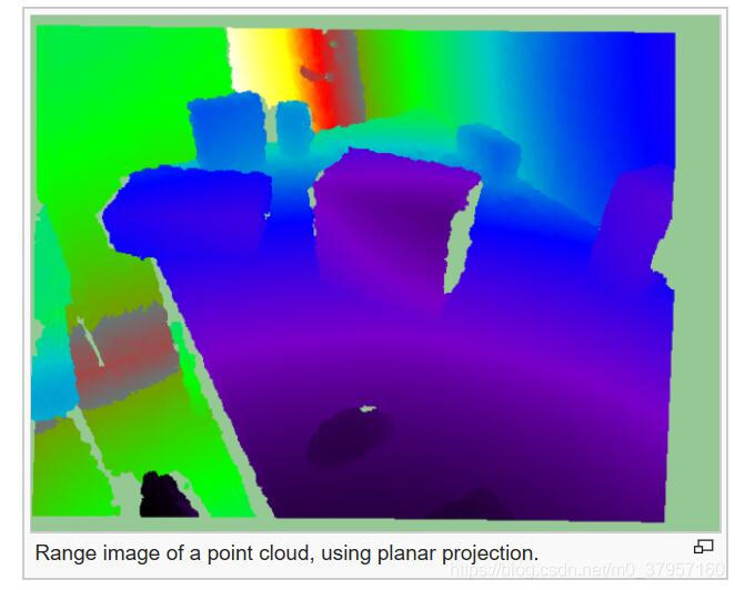
The Normal Aligned Radial Feature is the only descriptor here that does not take a point cloud as input. Instead, it works with range images. A range image is a common RGB image in which the distance to the point that corresponds to a certain pixel is encoded as a color value in the visible light spectrum: the points that are closer to the camera would be violet, while the points near the maximum sensor range would be red.

NARF also requires us to find suitable keypoints to compute the descriptor for. NARF keypoints are located near an object's corners, and this also requires to find the borders (transitions from foreground to background), which are trivial to find with a range image. Because of this lengthy pipeline, I will describe the whole process in different sections.

Obtaining a range image

Because we always work with point clouds, I will now explain how you can convert one into a range image, in order to use it for the NARF descriptor. PCL provides a couple of handy classes to perform the conversion, given that you fill the camera data correctly.

A range image can be created in two ways. First, we can use spherical projection, which would give us an image similar to the ones produced by a LIDAR sensor. Second, we can use planar projection, which is better suitable for camera-like sensors as the Kinect or the Xtion, and will not have the characteristic distortion of the first one.

Spherical projection

The following code will take a point cloud and create a range image from it, using spherical projection:

#include <pcl/io/pcd_io.h>
#include <pcl/range_image/range_image.h>
#include <pcl/visualization/range_image_visualizer.h>

int
main(int argc, char** argv)
{
	// Object for storing the point cloud.
	pcl::PointCloud<pcl::PointXYZ>::Ptr cloud(new pcl::PointCloud<pcl::PointXYZ>);

	// Read a PCD file from disk.
	if (pcl::io::loadPCDFile<pcl::PointXYZ>(argv[1], *cloud) != 0)
	{
		return -1;
	}

	// Parameters needed by the range image object:

	// Angular resolution is the angular distance between pixels.
	// Kinect: 57° horizontal FOV, 43° vertical FOV, 640x480 (chosen here).
	// Xtion: 58° horizontal FOV, 45° vertical FOV, 640x480.
	float angularResolutionX = (float)(57.0f / 640.0f * (M_PI / 180.0f));
	float angularResolutionY = (float)(43.0f / 480.0f * (M_PI / 180.0f));
	// Maximum horizontal and vertical angles. For example, for a full panoramic scan,
	// the first would be 360º. Choosing values that adjust to the real sensor will
	// decrease the time it takes, but don't worry. If the values are bigger than
	// the real ones, the image will be automatically cropped to discard empty zones.
	float maxAngleX = (float)(60.0f * (M_PI / 180.0f));
	float maxAngleY = (float)(50.0f * (M_PI / 180.0f));
	// Sensor pose. Thankfully, the cloud includes the data.
	Eigen::Affine3f sensorPose = Eigen::Affine3f(Eigen::Translation3f(cloud->sensor_origin_[0],
								 cloud->sensor_origin_[1],
								 cloud->sensor_origin_[2])) *
								 Eigen::Affine3f(cloud->sensor_orientation_);
	// Noise level. If greater than 0, values of neighboring points will be averaged.
	// This would set the search radius (e.g., 0.03 == 3cm).
	float noiseLevel = 0.0f;
	// Minimum range. If set, any point closer to the sensor than this will be ignored.
	float minimumRange = 0.0f;
	// Border size. If greater than 0, a border of "unobserved" points will be left
	// in the image when it is cropped.
	int borderSize = 1;

	// Range image object.
	pcl::RangeImage rangeImage;
	rangeImage.createFromPointCloud(*cloud, angularResolutionX, angularResolutionY,
									maxAngleX, maxAngleY, sensorPose, pcl::RangeImage::CAMERA_FRAME,
									noiseLevel, minimumRange, borderSize);

	// Visualize the image.
	pcl::visualization::RangeImageVisualizer viewer("Range image");
	viewer.showRangeImage(rangeImage);
	while (!viewer.wasStopped())
	{
		viewer.spinOnce();
		// Sleep 100ms to go easy on the CPU.
		pcl_sleep(0.1);
	}
}

Here you can see an example of the output range image:

Input: Points, Angular resolution, Maximum angle, Sensor pose, Coordinate frame, Noise level, Maximum range, Border size
Output: Range image (spherical projection)
Tutorials:
- How to create a range image from a point cloud
- How to visualize a range image
API: pcl::RangeImage
Download

10）Planar projection

As mentioned, planar projection will give better results with clouds taken from a depth camera:

#include <pcl/io/pcd_io.h>
#include <pcl/range_image/range_image_planar.h>
#include <pcl/visualization/range_image_visualizer.h>

int
main(int argc, char** argv)
{
	// Object for storing the point cloud.
	pcl::PointCloud<pcl::PointXYZ>::Ptr cloud(new pcl::PointCloud<pcl::PointXYZ>);

	// Read a PCD file from disk.
	if (pcl::io::loadPCDFile<pcl::PointXYZ>(argv[1], *cloud) != 0)
	{
		return -1;
	}

	// Parameters needed by the planar range image object:

	// Image size. Both Kinect and Xtion work at 640x480.
	int imageSizeX = 640;
	int imageSizeY = 480;
	// Center of projection. here, we choose the middle of the image.
	float centerX = 640.0f / 2.0f;
	float centerY = 480.0f / 2.0f;
	// Focal length. The value seen here has been taken from the original depth images.
	// It is safe to use the same value vertically and horizontally.
	float focalLengthX = 525.0f, focalLengthY = focalLengthX;
	// Sensor pose. Thankfully, the cloud includes the data.
	Eigen::Affine3f sensorPose = Eigen::Affine3f(Eigen::Translation3f(cloud->sensor_origin_[0],
								 cloud->sensor_origin_[1],
								 cloud->sensor_origin_[2])) *
								 Eigen::Affine3f(cloud->sensor_orientation_);
	// Noise level. If greater than 0, values of neighboring points will be averaged.
	// This would set the search radius (e.g., 0.03 == 3cm).
	float noiseLevel = 0.0f;
	// Minimum range. If set, any point closer to the sensor than this will be ignored.
	float minimumRange = 0.0f;

	// Planar range image object.
	pcl::RangeImagePlanar rangeImagePlanar;
	rangeImagePlanar.createFromPointCloudWithFixedSize(*cloud, imageSizeX, imageSizeY,
			centerX, centerY, focalLengthX, focalLengthX,
			sensorPose, pcl::RangeImage::CAMERA_FRAME,
			noiseLevel, minimumRange);

	// Visualize the image.
	pcl::visualization::RangeImageVisualizer viewer("Planar range image");
	viewer.showRangeImage(rangeImagePlanar);
	while (!viewer.wasStopped())
	{
		viewer.spinOnce();
		// Sleep 100ms to go easy on the CPU.
		pcl_sleep(0.1);
	}
}

Input: Points, Image size, Projection center, Focal length, Sensor pose, Coordinate frame, Noise level, Maximum range
Output: Range image (planar projection)
Tutorials:
- How to create a range image from a point cloud
- How to visualize a range image
API: pcl::RangeImagePlanar
Download

If you prefer to do the conversion in real time while you inspect the cloud, PCL ships with an example that fetches an "openni_wrapper::DepthImage" from an OpenNI device and creates the range image from it. You can adapt the code of the example example from tutorial 1 to save it to disk with the function pcl::io::saveRangeImagePlanarFilePNG().

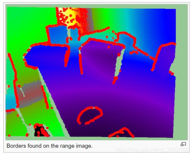
11）Extracting borders

NARF keypoints are located near the edges of objects in the range image, so in order to find them, we first have to extract the borders. A border is defined as an abrupt change from foreground to background. In a range image, this can be easily seen because there is a "jump" in the depth value of two adjacent pixels.

There are three types of borders. Object borders consist of the pixels (or points) located on the very edge of an object (the outermost points still belonging to the object). Shadow borders are points in the background on the edge of occlusions (empty areas in the background due to the objects in front covering them). Notice that, when the cloud is seen from the sensor's viewpoint, object and shadow points will seem adjacent. Finally, veil points are points interpolated between the previous two which appear in scans taken with LIDAR sensors, so we do not have to worry about them here.

The algorithm basically compares a point's depth with the values of its neighbors, and if a big difference is found, we know it is due to a border. Points closer to the sensor will be marked as object borders, and the other ones as shadow borders.

PCL provides a class for extracting borders of a range image:

#include <pcl/io/pcd_io.h>
#include <pcl/range_image/range_image_planar.h>
#include <pcl/features/range_image_border_extractor.h>
#include <pcl/visualization/range_image_visualizer.h>

int
main(int argc, char** argv)
{
	// Object for storing the point cloud.
	pcl::PointCloud<pcl::PointXYZ>::Ptr cloud(new pcl::PointCloud<pcl::PointXYZ>);
	// Object for storing the borders.
	pcl::PointCloud<pcl::BorderDescription>::Ptr borders(new pcl::PointCloud<pcl::BorderDescription>);

	// Read a PCD file from disk.
	if (pcl::io::loadPCDFile<pcl::PointXYZ>(argv[1], *cloud) != 0)
	{
		return -1;
	}

	// Convert the cloud to range image.
	int imageSizeX = 640, imageSizeY = 480;
	float centerX = (640.0f / 2.0f), centerY = (480.0f / 2.0f);
	float focalLengthX = 525.0f, focalLengthY = focalLengthX;
	Eigen::Affine3f sensorPose = Eigen::Affine3f(Eigen::Translation3f(cloud->sensor_origin_[0],
								 cloud->sensor_origin_[1],
								 cloud->sensor_origin_[2])) *
								 Eigen::Affine3f(cloud->sensor_orientation_);
	float noiseLevel = 0.0f, minimumRange = 0.0f;
	pcl::RangeImagePlanar rangeImage;
	rangeImage.createFromPointCloudWithFixedSize(*cloud, imageSizeX, imageSizeY,
			centerX, centerY, focalLengthX, focalLengthX,
			sensorPose, pcl::RangeImage::CAMERA_FRAME,
			noiseLevel, minimumRange);

	// Border extractor object.
	pcl::RangeImageBorderExtractor borderExtractor(&rangeImage);

	borderExtractor.compute(*borders);

	// Visualize the borders.
	pcl::visualization::RangeImageVisualizer* viewer = NULL;
	viewer = pcl::visualization::RangeImageVisualizer::getRangeImageBordersWidget(rangeImage,
			 -std::numeric_limits<float>::infinity(),
			 std::numeric_limits<float>::infinity(),
			 false, *borders, "Borders");

	while (!viewer->wasStopped())
	{
		viewer->spinOnce();
		// Sleep 100ms to go easy on the CPU.
		pcl_sleep(0.1);
	}
}

You can use the extractor's "getParameters()" function to get a pcl::RangeImageBorderExtractor::Parameters struct with the settings that will be used.

Input: Range image
Output: Borders
Tutorial: How to extract borders from range images
Publication:
- Point Feature Extraction on 3D Range Scans Taking into Account Object Boundaries (Bastian Steder et al., 2011)
API: pcl::RangeImageBorderExtractor
Download

12）Finding keypoints

Citing the original publication: 文章链接见：

"We have the following requirements for our interest point extraction procedure:

It must take information about borders and the surface structure into account.
It must select positions that can be reliably detected even if the object is observed from another perspective.
The points must be on positions that provide stable areas for normal estimation or the descriptor calculation in general."

The procedure is the following: for every point in the range image, a score is computed that conveys how much the surface changes in its neighborhood (this is tuned with the support size σ, which is the diameter of the sphere used to find neighboring points). Also, the dominant direction of this change is computed. Then, this direction is compared with those of the neighbors, trying to find how stable the point is (if the directions are very different, that means the point is not stable, and that the surface around changes a lot). Points that are near the object's corners (but not exactly on the very edge) will be good keypoints, yet stable enough.

In PCL, NARF keypoints can be found this way:

#include <pcl/io/pcd_io.h>
#include <pcl/range_image/range_image_planar.h>
#include <pcl/features/range_image_border_extractor.h>
#include <pcl/keypoints/narf_keypoint.h>
#include <pcl/visualization/range_image_visualizer.h>

int
main(int argc, char** argv)
{
	// Object for storing the point cloud.
	pcl::PointCloud<pcl::PointXYZ>::Ptr cloud(new pcl::PointCloud<pcl::PointXYZ>);
	// Object for storing the keypoints' indices.
	pcl::PointCloud<int>::Ptr keypoints(new pcl::PointCloud<int>);

	// Read a PCD file from disk.
	if (pcl::io::loadPCDFile<pcl::PointXYZ>(argv[1], *cloud) != 0)
	{
		return -1;
	}

	// Convert the cloud to range image.
	int imageSizeX = 640, imageSizeY = 480;
	float centerX = (640.0f / 2.0f), centerY = (480.0f / 2.0f);
	float focalLengthX = 525.0f, focalLengthY = focalLengthX;
	Eigen::Affine3f sensorPose = Eigen::Affine3f(Eigen::Translation3f(cloud->sensor_origin_[0],
								 cloud->sensor_origin_[1],
								 cloud->sensor_origin_[2])) *
								 Eigen::Affine3f(cloud->sensor_orientation_);
	float noiseLevel = 0.0f, minimumRange = 0.0f;
	pcl::RangeImagePlanar rangeImage;
	rangeImage.createFromPointCloudWithFixedSize(*cloud, imageSizeX, imageSizeY,
			centerX, centerY, focalLengthX, focalLengthX,
			sensorPose, pcl::RangeImage::CAMERA_FRAME,
			noiseLevel, minimumRange);

	pcl::RangeImageBorderExtractor borderExtractor;
	// Keypoint detection object.
	pcl::NarfKeypoint detector(&borderExtractor);
	detector.setRangeImage(&rangeImage);
	// The support size influences how big the surface of interest will be,
	// when finding keypoints from the border information.
	detector.getParameters().support_size = 0.2f;

	detector.compute(*keypoints);

	// Visualize the keypoints.
	pcl::visualization::RangeImageVisualizer viewer("NARF keypoints");
	viewer.showRangeImage(rangeImage);
	for (size_t i = 0; i < keypoints->points.size(); ++i)
	{
		viewer.markPoint(keypoints->points[i] % rangeImage.width,
						 keypoints->points[i] / rangeImage.width,
						 // Set the color of the pixel to red (the background
						 // circle is already that color). All other parameters
						 // are left untouched, check the API for more options.
						 pcl::visualization::Vector3ub(1.0f, 0.0f, 0.0f));
	}

	while (!viewer.wasStopped())
	{
		viewer.spinOnce();
		// Sleep 100ms to go easy on the CPU.
		pcl_sleep(0.1);
	}
}

Input: Range image, Border extractor, Support Size
Output: NARF keypoints
Tutorial: How to extract NARF keypoint from a range image
Publication:
- Point Feature Extraction on 3D Range Scans Taking into Account Object Boundaries (Bastian Steder et al., 2011)
API: pcl::NarfKeypoint
Download

13）Computing the descriptor

We have created the range image from a point cloud, and we have extracted the borders in order to find good keypoints. Now it is time to compute the NARF descriptor for each keypoint.

The NARF descriptor encodes information about surface changes around a point. First, a local range patch is created around the point. It is like a small range image centered at that point, aligned with the normal (it would seem as if we were looking at the point along the normal). Then, a star pattern with n beams is overlaid onto the patch, also centered at the point. For every beam, a value is computed, that reflects how much the surface under it changes. The stronger the change is, and the closer to the center it is, the higher the final value will be. The n resulting values compose the final descriptor.

The descriptor right now is not invariant to rotations around the normal. To achieve this, the whole possible 360 degrees are binned into an histogram. The value of each bin is computed from the descriptor values according to the angle. Then, the bin with the highest value is considered the dominant orientation, and the descriptor is shifted according to it.

#include <pcl/io/pcd_io.h>
#include <pcl/range_image/range_image_planar.h>
#include <pcl/features/range_image_border_extractor.h>
#include <pcl/keypoints/narf_keypoint.h>
#include <pcl/features/narf_descriptor.h>

int
main(int argc, char** argv)
{
	// Object for storing the point cloud.
	pcl::PointCloud<pcl::PointXYZ>::Ptr cloud(new pcl::PointCloud<pcl::PointXYZ>);
	// Object for storing the keypoints' indices.
	pcl::PointCloud<int>::Ptr keypoints(new pcl::PointCloud<int>);
	// Object for storing the NARF descriptors.
	pcl::PointCloud<pcl::Narf36>::Ptr descriptors(new pcl::PointCloud<pcl::Narf36>);

	// Read a PCD file from disk.
	if (pcl::io::loadPCDFile<pcl::PointXYZ>(argv[1], *cloud) != 0)
	{
		return -1;
	}

	// Convert the cloud to range image.
	int imageSizeX = 640, imageSizeY = 480;
	float centerX = (640.0f / 2.0f), centerY = (480.0f / 2.0f);
	float focalLengthX = 525.0f, focalLengthY = focalLengthX;
	Eigen::Affine3f sensorPose = Eigen::Affine3f(Eigen::Translation3f(cloud->sensor_origin_[0],
								 cloud->sensor_origin_[1],
								 cloud->sensor_origin_[2])) *
								 Eigen::Affine3f(cloud->sensor_orientation_);
	float noiseLevel = 0.0f, minimumRange = 0.0f;
	pcl::RangeImagePlanar rangeImage;
	rangeImage.createFromPointCloudWithFixedSize(*cloud, imageSizeX, imageSizeY,
			centerX, centerY, focalLengthX, focalLengthX,
			sensorPose, pcl::RangeImage::CAMERA_FRAME,
			noiseLevel, minimumRange);

	// Extract the keypoints.
	pcl::RangeImageBorderExtractor borderExtractor;
	pcl::NarfKeypoint detector(&borderExtractor);
	detector.setRangeImage(&rangeImage);
	detector.getParameters().support_size = 0.2f;
	detector.compute(*keypoints);

	// The NARF estimator needs the indices in a vector, not a cloud.
	std::vector<int> keypoints2;
	keypoints2.resize(keypoints->points.size());
	for (unsigned int i = 0; i < keypoints->size(); ++i)
		keypoints2[i] = keypoints->points[i];
	// NARF estimation object.
	pcl::NarfDescriptor narf(&rangeImage, &keypoints2);
	// Support size: choose the same value you used for keypoint extraction.
	narf.getParameters().support_size = 0.2f;
	// If true, the rotation invariant version of NARF will be used. The histogram
	// will be shifted according to the dominant orientation to provide robustness to
	// rotations around the normal.
	narf.getParameters().rotation_invariant = true;

	narf.compute(*descriptors);
}

Input: Range image, Key points, Support Size
Output: NARF descriptors
Tutorial: How to extract NARF Features from a range image
Publication:
- Point Feature Extraction on 3D Range Scans Taking into Account Object Boundaries (Bastian Steder et al., 2011)
API: pcl::NarfDescriptor
Download

14）RoPS

The Rotational Projection Statistics (RoPS) feature is a bit different from the other descriptors because it works with a triangle mesh, so a previous triangulation step is needed for generating this mesh from the cloud. Apart from that, most concepts are similar.

In order to compute RoPS for a keypoint, the local surface is cropped according to a support radius, so only points and triangles lying inside are taken into account. Then, a local reference frame (LRF) is computed, giving the descriptor its rotational invariance. A coordinate system is created with the point as the origin, and the axes aligned with the LRF. Then, for every axis, several steps are performed.

First, the local surface is rotated around the current axis. The angle is determined by one of the parameters, which sets the number of rotations. Then, all points in the local surface are projected onto the XY, XZ and YZ planes. For each one, statistical information about the distribution of the projected points is computed, and concatenated to form the final descriptor.

#include <pcl/io/pcd_io.h>
#include <pcl/point_types_conversion.h>
#include <pcl/features/normal_3d.h>
#include <pcl/surface/gp3.h>
#include <pcl/features/rops_estimation.h>

// A handy typedef.
typedef pcl::Histogram<135> ROPS135;

int
main(int argc, char** argv)
{
	// Object for storing the point cloud.
	pcl::PointCloud<pcl::PointXYZ>::Ptr cloud(new pcl::PointCloud<pcl::PointXYZ>);
	// Object for storing the normals.
	pcl::PointCloud<pcl::Normal>::Ptr normals(new pcl::PointCloud<pcl::Normal>);
	// Object for storing both the points and the normals.
	pcl::PointCloud<pcl::PointNormal>::Ptr cloudNormals(new pcl::PointCloud<pcl::PointNormal>);
	// Object for storing the ROPS descriptor for each point.
	pcl::PointCloud<ROPS135>::Ptr descriptors(new pcl::PointCloud<ROPS135>());

	// Read a PCD file from disk.
	if (pcl::io::loadPCDFile<pcl::PointXYZ>(argv[1], *cloud) != 0)
	{
		return -1;
	}

	// Estimate the normals.
	pcl::NormalEstimation<pcl::PointXYZ, pcl::Normal> normalEstimation;
	normalEstimation.setInputCloud(cloud);
	normalEstimation.setRadiusSearch(0.03);
	pcl::search::KdTree<pcl::PointXYZ>::Ptr kdtree(new pcl::search::KdTree<pcl::PointXYZ>);
	normalEstimation.setSearchMethod(kdtree);
	normalEstimation.compute(*normals);

	// Perform triangulation.
	pcl::concatenateFields(*cloud, *normals, *cloudNormals);
	pcl::search::KdTree<pcl::PointNormal>::Ptr kdtree2(new pcl::search::KdTree<pcl::PointNormal>);
	kdtree2->setInputCloud(cloudNormals);
	pcl::GreedyProjectionTriangulation<pcl::PointNormal> triangulation;
	pcl::PolygonMesh triangles;
	triangulation.setSearchRadius(0.025);
	triangulation.setMu(2.5);
	triangulation.setMaximumNearestNeighbors(100);
	triangulation.setMaximumSurfaceAngle(M_PI / 4); // 45 degrees.
	triangulation.setNormalConsistency(false);
	triangulation.setMinimumAngle(M_PI / 18); // 10 degrees.
	triangulation.setMaximumAngle(2 * M_PI / 3); // 120 degrees.
	triangulation.setInputCloud(cloudNormals);
	triangulation.setSearchMethod(kdtree2);
	triangulation.reconstruct(triangles);

	// Note: you should only compute descriptors for chosen keypoints. It has
	// been omitted here for simplicity.

	// RoPs estimation object.
	pcl::ROPSEstimation<pcl::PointXYZ, ROPS135> rops;
	rops.setInputCloud(cloud);
	rops.setSearchMethod(kdtree);
	rops.setRadiusSearch(0.03);
	rops.setTriangles(triangles.polygons);
	// Number of partition bins that is used for distribution matrix calculation.
	rops.setNumberOfPartitionBins(5);
	// The greater the number of rotations is, the bigger the resulting descriptor.
	// Make sure to change the histogram size accordingly.
	rops.setNumberOfRotations(3);
	// Support radius that is used to crop the local surface of the point.
	rops.setSupportRadius(0.025);

	rops.compute(*descriptors);
}

Input: Points, Triangles, Search method, Support radius, Number of rotations, Number of partition bins
Output: RoPS descriptors
Publication:
- Rotational Projection Statistics for 3D Local Surface Description and Object Recognition (Yulan Guo et al., 2013)
API: pcl::ROPSEstimation
Download

Global descriptors

Global descriptors encode object geometry. They are not computed for individual points, but for a whole cluster that represents an object. Because of this, a preprocessing step (segmentation) is required, in order to retrieve possible candidates.

Global descriptors are used for object recognition and classification, geometric analysis (object type, shape...), and pose estimation.

You should also know that many local descriptors can also be used as global ones. This can be done with descriptors that use a radius to search for neighbors (as PFH does). The trick is to compute it for one single point in the object cluster, and set the radius to the maximum possible distance between any two points (so all points in the cluster are considered as neighbors).