Tensorflow 笔记 Ⅺ——NLP 实现电影评论情感分析

特别说明

•此次博客仅使用 TensorFlow 2.x 进行，但在使用 TensorFlow 2.x 的同时使用了两种方式，一种是利用 TensorFlow 2.x 高阶 API Keras 自动读取数据集，一种是下载原始数据集进行数据提取，其中处理原始数据集的方式就适用于TensorFlow1.x，两者没有本质的区别
•本次未适用 TensorFlow 的低阶 API，笔者水平有限，现在还未涉及如何使用 TensorFlow 低阶 API 搭建 RNN(LSTM)网络，后期应该会有做这一方面博客的打算

数据集

IMDB 简介

互联网电影资料库（Internet Movie Database，简称IMDb）是一个关于电影演员、电影、电视节目、电视明星和电影制作的在线数据库。
•IMDb创建于1990年10月17日，从1998年开始成为亚马逊公司旗下网站，2010年是IMDb成立20周年纪念。
•IMDb的资料中包括了影片的众多信息、演员、片长、内容介绍、分级、评论等。对于电影的评分目前使用最多的就是IMDb评分。
•截至2018年6月21日，IMDb共收录了4,734,693部作品资料以及8,702,001名人物资料。
•IMDb不只是电影和电子游戏的数据库，还提供每日更新的电影电视新闻，以及为不同电影活动比如奥斯卡奖推出特别报道。IMDb的论坛也十分活跃，除每个数据库条目都有留言板之外，还有关于多种多样的主题的各种综合讨论版。为此提供了经典的电影评论的数据集 IMDB
IMDB 官网

IMDB 数据集

下载地址

斯坦福大学人工智能实验室的IMDb影评数据集：
http://ai.stanford.edu/~amaas/data/sentiment/

具体数据文件URL：
http://ai.stanford.edu/~amaas/data/sentiment/aclImdb_v1.tar.gz

目录结构

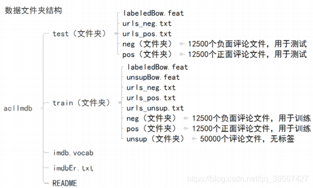
IMDb数据集可用于二分类的情感分析主要分为两部分：

数据	含义
训练数据	25000个评论（正面评论与负面评论各12500个）
测试数据	25000个评论（正面评论与负面评论各12500个）

其文件目录结构如下

其中 train，test 下才存放了真正的评论文本，urls 则存放了评论文本的地址

示例文本

Once again Mr. Costner has dragged out a movie for far longer than necessary. Aside from the terrific sea rescue sequences, of which there are very few I just did not care about any of the characters. Most of us have ghosts in the closet, and Costner’s character are realized early on, and then forgotten until much later, by which time I did not care. The character we should really care about is a very cocky, overconfident Ashton Kutcher. The problem is he comes off as kid who thinks he’s better than anyone else around him and shows no signs of a cluttered closet. His only obstacle appears to be winning over Costner. Finally when we are well past the half way point of this stinker, Costner tells us all about Kutcher’s ghosts. We are told why Kutcher is driven to be the best with no prior inkling or foreshadowing. No magic here, it was all I could do to keep from turning it off an hour in.

译文来源 Google Translate
Costner先生再一次拖延电影的放映时间远远超过了必要。 除了出色的海上救援工作，我很少在乎其中的任何角色。 我们大多数人的壁橱里都有鬼魂，科斯特纳的性格很早就意识到了，然后被遗忘到很晚，那时我不在乎。 我们真正应该关心的角色是一个非常自大，过分自信的Ashton Kutcher。 问题是他从小就离开了，他认为自己比周围的任何人都要好，而且没有壁橱混乱的迹象。 他唯一的障碍似乎是要击败科斯特纳。 最终，当我们远远超过了臭鼬的中间点时，科斯特纳向我们讲述了库奇的幽灵。 有人告诉我们，为什么Kutcher在没有事先征兆或预先埋头的情况下被驱使成为最好的人。 这里没有什么魔力，这是我能做的一切，避免在一小时内关闭它。

可以看出这是一条差评，正好这段文本复制于 aclImdb\test\neg\0_2.txt

自然语言处理基础

分词

分词是文本，或者说是一段话的特征，我们在平时考试都知道在阅读时要找取关键字，关键词，而关键字关键词就是被我们读者划分出来的（机器也需要划分），给机器分词就是一个复杂的研究领域，汉语作为世界上最复杂的语言，分词也是最复杂的例如一下五个句子，别说机器了，就是人说快了也是听的一脸懵逼

1.今天下雨，我骑车差点摔倒，好在我一把/把把/把住了！
2.来到杨过曾经生zhidao活的地方，小龙女动情地说：“我也想过过/过儿/过过/的生活。”
3.多亏跑了两步，差点没上上/上/上海的车。
4.用毒内/毒/毒蛇/毒蛇会不会容被毒/毒死？
5.校长说：校服上除了校徽别别/别的，让你们别别/别的/别别/别的你非得别/别的！

自然语言处理常见特征
• 单独词
• 词的n元组
• 单独词或n元组出现的频率
• 词的词性
• 词的位置
……
想从文本中提取特征，分词非常重要

Python的中文分词库：jieba（结巴分词）、THULAC（清华大学自然语言处理与社会人文计算实验室）、pkuseg（北京大学语言计算与机器学习研究组）

词的数字化表示方法与词嵌入

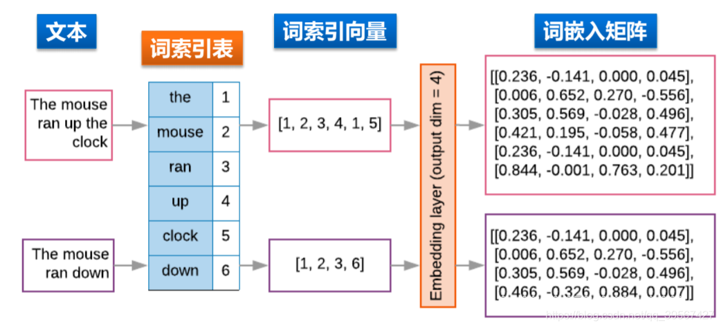
在前面的一些深度学习模型中，无论是图像的处理还是像 boston 房价的文件，我们都将其进行了预处理，其中重要的一步就是数字化，因为计算机只认得二进制，所以我们需要将一些字符串进行数字化，所以词嵌入就是解决词与数字的映射关系，对文本的处理可分为两步：
• 1.将文本分词处理，并将分词与数字形成映射关系
• 2.将每一个分词用独特的向量进行表示，这样文本中的每一个分词就是一个向量，每一个向量一起构成文本，这就将文本转换成了二维矩阵，在构建 IMDB 的模型时，我们也将遵循这一规则

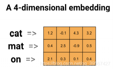
词嵌入（word embedding）
一个词嵌入是一个稠密浮点数向量（向量长度可以设置），它们是可以训练的参数，一般词嵌入是8维（对于小型数据集）到1024维（大型数据集），更高的维度嵌入可以捕获词之间更细的关系，但是需要更多数据去学习

例如一个四维的词嵌入，每一个分词用一个四维向量代替

词嵌入模型
词嵌入的模型可以自己训练也可以使用成熟的预训练模型，常见的词嵌入模型有word2vec、GloVe等(都是英文词)

Version	说明
word2vec	通过对具有数十亿词的新闻文章进行训练，Google提供了一组词向量的结果，可点击链接获取(好像失效了)
GloVe	如果想要训练中文文本，这里有一些预训练的中文词嵌入可用： https://github.com/Embedding/Chinese-Word-Vectors

为此词嵌入步骤一图以蔽之

循环神经网络 RNN与LSTM

数据的时序与含义

很多问题具有时序性，自然语言处理、视频图像处理、股票交易信息等等
例如：

昨天晚上我在超市买了一袋酸菜牛肉面，今天下午午饭过后，博客写着有点饿了，我于是就泡了一碗泡面吃

根据全语句可以很明显的知道，泡的这碗泡面很有可能就是酸菜牛肉面，如果没有前面的语句，可能就只能瞎猜了，所以时序在自然语言处理尤为重要，多层全连接的神经网络或者卷积神经网络都只能根据当前的状态进行处理，不能很好地处理时序问题

RNN的模型结构（Recurrent Neural Network）

RNN 网络展开图

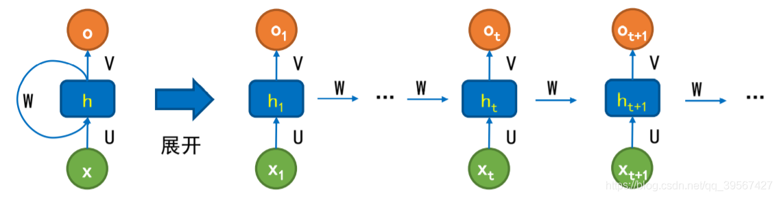
可以清楚的发现，传递下一个时刻的参数来源于前面多个时刻，而全连接神经网络参数的更新仅仅根据当前状态，其中的参数表示如下
隐含层： $h_t=f(W_{ht}-1+U_{xt}+b_h)$
输出层： $ot=g(V_{ht}+b_o)$

可以从递推时看出，参数之间属于乘积关系，这里就有个致命的弱点，在反向传播求梯度中，如果某一次更新使得权值 $W_{ht}$过大，那么就会使得输出也偏大，如果没有控制，输入进下一个时刻的参数就会变大，使得 $W_{ht}$ 变的更大，这就会让权值越界造成梯度爆炸(接近正无穷)，同理如果 $W_{ht}$ 变的很小，就会造成梯度消失(接近于 0)，这是由于在 RNN 中我们长使用的激活函数为 $tanh$， $tanh$ 的倒数在 0~1，且还是偶函数

$tanh(red), tanh'(green)$

RNN可以将之前处理的信息与当前节点联系起来，所以它可以处理序列问题但是当序列过长时，由于梯度消失和梯度爆炸问题，对于 $t$ 时刻来说，它产生的梯度在时间轴上向历史传播几层之后就消失了，根本就无法影响太遥远的过去。“所有历史”共同作用只是理想的情况，在实际中，这种影响也就只能维持若干个时间戳。RNN会忘记很久以前出现的信息，而只能记住近期出现的信息，所以RNN很难有效处理长文本

LSTM（Long Short-Term Memory 长短时记忆网络）

传统RNN每一步的隐藏单元只是执行一个简单的tanh或ReLU操作，LSTM基本结构和RNN相似，主要不同是LSTM对隐含层进行了改进在LSMT中，每个神经元相当于一个记忆细胞（Cell）

基本状态

LSTM的关键是细胞的状态，细胞的状态类似于传送带，直接在整个链路上运行，只有一些少量的线性交互

遗忘门

决定丢弃上一步的哪些信息
该门会读取 $h_{t−1}$ 和 $x_t$，输出一个在 0 到 1 之间的数值给每个在细胞状态 $C_{t−1}$ 中的数字。1 表示“完全保留”，0 表示“完全舍弃”

$ft=σ(W_f•[h_{t-1},x_t]+b_f)$

输入门

决定加入哪些新的信息
$tanh$ 层创建一个新的候选值向量 $\widetilde{C_t}$，加到状态中。这里sigmoid层称“输入门层”，起到一个缩放的作用。这两个信息产生对状态的更新

$i_t=σ(W_i•[h_{t-1},x_t]+b_i), \widetilde{C_t}=tanh(W_c•[h_{t-1},x_t]+b_c)$

形成新的细胞状态

1.旧的细胞状态 $C_{t−1}$ 与 $f_t$ 相乘来丢弃一部分信息
2.再加上 $i_t• \widetilde{C_t}$（ $i$ 是input输入门），生成新的细胞状态 $C_t$

$c_t=f_t•C_{t−1}+i_t•\widetilde{C_t}$

输出门

决定输出哪些信息
把 $C_t$ 输给 $tanh$ 函数，得到一个候选的输出值，运行一个 $sigmoid$ 层来确定细胞状态的哪个部分将输出出去

$o_t=σ(W_o•[h_{t-1},xt]+b_o),h_t=o_t•tanh(C_t)$

LSTM优势

LSTM相比于RNN的优点：
1.梯度下降法中，RNN的梯度求解是累乘的形式，由于LSTM的隐含层更复杂，LSTM在梯度求解时，式子是累加的形式，所以LSTM的梯度往往不会是一个接近于0的小值，缓解了梯度消失的问题
2. 使用了门结构，解决了长距离依赖的问题

IMDB 情感分析 TensorFLow 2.x 实现

前情函数

tf.keras.preprocessing.sequence.pad_sequences

tf.keras.preprocessing.sequence.pad_sequences(
    sequences, maxlen=None, dtype=‘int32’, padding=‘pre’, truncating=‘pre’,
    value=0.0
)
此函数将一个整数列表转换为维度为 2D 的 Numpy 数组，maxlen 变量值确定列表中最长序列的长度，若序列是短于指定长度将被填充到指定长度，若序列的长度长于指定长度将被截取到指定长度，填充或截断发生的位置分别由参数 padding 和决定 truncating。默认填充是从序列开始处预填充或删除值


参数:
    sequences：序列列表（每个序列都必须是整数列表）
    maxlen：可选Int，所有序列的最大长度。如果未提供，则将序列填充为最长的单个序列的长度
    dtype：（可选，默认为int32）。输出序列的类型。要填充长度可变的字符串序列，可以使用object
    padding：字符串，pre 或 post（可选，默认为 pre）：在每个序列之前或之后填充
    truncating：字符串，pre 或 post（可选，默认为 pre）：从序列中大于 maxlen 或等于的序列的开头或结尾删除值，post 则是从末尾操作
    value：浮点型或字符串型，填充值。（可选，默认为0。）
返回值:
    Numpy 数组，shape=(len(sequences), maxlen)

默认选取最长的列表元素为准
默认填充值为 0
默认填充方式为 pre（从前填充）

import tensorflow as tf

sequence = [[1], [2, 3], [4, 5, 6]] 
tf.keras.preprocessing.sequence.pad_sequences(sequence)

array([[0, 0, 1],
       [0, 2, 3],
       [4, 5, 6]])

指定填充 -1

tf.keras.preprocessing.sequence.pad_sequences(sequence, value=-1) 

array([[-1, -1,  1],
       [-1,  2,  3],
       [ 4,  5,  6]])

指定填充模式为从后填充

tf.keras.preprocessing.sequence.pad_sequences(sequence, padding='post') 

array([[1, 0, 0],
       [2, 3, 0],
       [4, 5, 6]])

指定最大序列长度为 2 且截断方式为 post，截断尾部操作，若为默认的 pre 操作，输出为
array([[0, 1],
      [2, 3],
      [4, 5]])

tf.keras.preprocessing.sequence.pad_sequences(sequence, maxlen=2, truncating='post') 

array([[0, 1],
       [2, 3],
       [4, 5]])

tf.keras.datasets.imdb.load_data

tf.keras.datasets.imdb.load_data(
    path=‘imdb.npz’, num_words=None, skip_top=0, maxlen=None, seed=113,
    start_char=1, oov_char=2, index_from=3, **kwargs
)
这里仅做简单介绍
参数:
    path：数据的缓存位置（相对于~/.keras/dataset）
    num_words：整数或无。根据单词出现的频率（在训练集中）对单词进行排名，并且仅保留 num_words 个最频繁出现的单词。频率较低的单词将在序列数据中显示为 oov_char 值。如果为None，将保留所有单词。(默认为无，因此保留所有单词)
    skip_top：跳过前N个最频繁出现的单词（可能没有参考意义）。这些单词将oov_char在数据集中显示为 值。默认值为0，因此不会跳过任何单词
    maxlen：int或无。最大序列长度。更长的序列将被截断。默认为无，表示没有截断
    seed：int 随机种子，用于随机打乱数据
    start_char：int 序列的开始将以该字符标记。默认为1，因为 0 通常是填充字符
    oov_char：int 言外之意。由于 num_words 或 skip_top限制而被删掉的单词将被替换为该字符
    index_from：int 用此索引和更高的索引索引实际单词
    **kwargs：用于向后兼容

返回值:
      Numpy数组的元组：(x_train, y_train), (x_test, y_test)


我们只需要指定 num_words 的值就行了，英文常用词汇大概在3000~5000，所以我们在读取数据时设定值为 5000，其中截长补短部分也可直接在数据读入时进行，但为了较统计学方式的设定值，我们利用 75% 的值作为 maxlen 的取值

# 统一文本长度，截长补短处代码
# x_train = tf.keras.preprocessing.sequence.pad_sequences(train_data,
#                              padding='post',
#                              truncating='post',
#                              maxlen=length)
# x_test = tf.keras.preprocessing.sequence.pad_sequences(test_data,
#                              padding='post',
#                              truncating='post',
#                              maxlen=length)

中文分词词库 jieba 使用初步

jieba 的命名是一个有趣的故事，跟‘结巴’同音，因为结巴说话就是结结巴巴一个词一个词的突出，首次使用时可使用!pip install jieba在 jupyter 实现安装


三种分词模式:
① 精确模式：试图将句子最精确地切开，适合文本分析
② 全模式：把句子中所有的可以成词的词语都扫描出来, 速度非常快，但是不能解决歧义
③ 搜索引擎模式：在精确模式的基础上，对长词再次切分，提高召回率，适合用于搜索引擎分词


特点:
• 支持繁体分词
• 支持自定义词典


其中支持自定义词典优点尤为突出，在处理一些特定情境会话时可以将专业名词划分出来

结巴分词使用
• jieba.cut 方法接受三个输入参数: 需要分词的字符串；cut_all 参数用来控制是否采用全模式；HMM 参数用来控制是否使用 HMM 模型
• jieba.cut_for_search 方法接受两个参数：需要分词的字符串；是否使用 HMM 模型。该方法适合用于搜索引擎构建倒排索引的分词
• jieba.cut 以及 jieba.cut_for_search 返回的结构都是一个可迭代的 generator，可以使用 for 循环来获得分词后得到的每一个词语，或者用jieba.lcut 以及 jieba.lcut_for_search 直接返回 list

import jieba

text = '我本科毕业于电子科技大学，现在已被保送电子科技大学硕士研究生'
print('文本信息:', text)

文本信息: 我本科毕业于电子科技大学，现在已被保送电子科技大学硕士研究生

注意: 直接使用 jieba.cut 需要 list 操作将 generator 转换为列表形式

word_list = jieba.cut(text)
print(list(word_list))

['我', '本科毕业', '于', '电子科技', '大学', '，', '现在', '已', '被', '保送', '电子科技', '大学', '硕士', '研究生']

使用 join 可以很好的适配 generator，精准模式直接分割文本信息

word_list = jieba.cut(text, cut_all=False)
print("精准模式分词结果为:" + "/".join(word_list))

精准模式分词结果为:我/本科毕业/于/电子科技/大学/，/现在/已/被/保送/电子科技/大学/硕士/研究生

全模式会把文本信息的每个词的所有可能组合进行输出

word_list = jieba.cut(text, cut_all=True)
print("全模式分词结果为:" + "/".join(word_list))

全模式分词结果为:我/本科/本科毕业/毕业/于/电子/电子科/电子科技/科技/大学/，/现在/已/被/保送/送电/电子/电子科/电子科技/科技/大学/硕士/研究/研究生

lcut 操作会把生成的 generator 自动转换为列表

word_list = jieba.lcut(text)
print(word_list)

['我', '本科毕业', '于', '电子科技', '大学', '，', '现在', '已', '被', '保送', '电子科技', '大学', '硕士', '研究生']

搜索引擎模式，类似搜索引擎一样组合并提取关键词

word_list = jieba.lcut_for_search(text)
print(word_list)

['我', '本科', '毕业', '本科毕业', '于', '电子', '科技', '电子科', '电子科技', '大学', '，', '现在', '已', '被', '保送', '电子', '科技', '电子科', '电子科技', '大学', '硕士', '研究', '研究生']

为了将电子科技大学作为一个专业名词采取自定义字典模式，其中也包括本科毕业词汇

with open('mydict.txt', 'w', encoding='utf-8') as file:
    file.write('电子科技大学\n本科毕业')

jieba.load_userdict('mydict.txt')

word_list = jieba.lcut(text)
print(word_list)

['我', '本科毕业', '于', '电子科技大学', '，', '现在', '已', '被', '保送', '电子科技大学', '硕士', '研究生']

全连接网络实现正式开始

import tensorflow as tf
import numpy as np
import matplotlib.pyplot as plt


tf.__version__

'2.0.0'

下载并装载数据集

TensorFlow2.x 读取的数据是已经装载并映射好的数据集，有关数据集的格式参见 TensorFlow1.x 如何将文字信息与数字信息映射的方法与步骤

imdb = tf.keras.datasets.imdb
(train_data, train_labels), (test_data, test_labels) = imdb.load_data(num_words=5000)

print('Training entries:{}, labels:{}'.format(len(train_data), len(train_labels)))

Training entries:25000, labels:25000

可以发现数据集为数字列表，共有 25000 个元素，当然测试数据也是如此

print('train detaset first value:\n', train_data[0],
      '\ntrain detaset first label:', train_labels[0],
      '\ntest detaset first value:\n', test_data[0],
      '\ntest detaset first label:', test_labels[0],)

train detaset first value:
 [1, 14, 22, 16, 43, 530, 973, 1622, 1385, 65, 458, 4468, 66, 3941, 4, 173, 36, 256, 5, 25, 100, 43, 838, 112, 50, 670, 2, 9, 35, 480, 284, 5, 150, 4, 172, 112, 167, 2, 336, 385, 39, 4, 172, 4536, 1111, 17, 546, 38, 13, 447, 4, 192, 50, 16, 6, 147, 2025, 19, 14, 22, 4, 1920, 4613, 469, 4, 22, 71, 87, 12, 16, 43, 530, 38, 76, 15, 13, 1247, 4, 22, 17, 515, 17, 12, 16, 626, 18, 2, 5, 62, 386, 12, 8, 316, 8, 106, 5, 4, 2223, 2, 16, 480, 66, 3785, 33, 4, 130, 12, 16, 38, 619, 5, 25, 124, 51, 36, 135, 48, 25, 1415, 33, 6, 22, 12, 215, 28, 77, 52, 5, 14, 407, 16, 82, 2, 8, 4, 107, 117, 2, 15, 256, 4, 2, 7, 3766, 5, 723, 36, 71, 43, 530, 476, 26, 400, 317, 46, 7, 4, 2, 1029, 13, 104, 88, 4, 381, 15, 297, 98, 32, 2071, 56, 26, 141, 6, 194, 2, 18, 4, 226, 22, 21, 134, 476, 26, 480, 5, 144, 30, 2, 18, 51, 36, 28, 224, 92, 25, 104, 4, 226, 65, 16, 38, 1334, 88, 12, 16, 283, 5, 16, 4472, 113, 103, 32, 15, 16, 2, 19, 178, 32] 
train detaset first label: 1 
test detaset first value:
 [1, 591, 202, 14, 31, 6, 717, 10, 10, 2, 2, 5, 4, 360, 7, 4, 177, 2, 394, 354, 4, 123, 9, 1035, 1035, 1035, 10, 10, 13, 92, 124, 89, 488, 2, 100, 28, 1668, 14, 31, 23, 27, 2, 29, 220, 468, 8, 124, 14, 286, 170, 8, 157, 46, 5, 27, 239, 16, 179, 2, 38, 32, 25, 2, 451, 202, 14, 6, 717] 
test detaset first label: 0

数据集预处理

由于网络输入数据必须是同维度，因此需要将得到的数据集或切割或填充的方法统一维度(也就是每一个数据列表的元素个数必须相同)

获取训练集列表元素排位在 75% 的长度，以此作为输入的维度

total = []
for i in range(len(train_data)):
    total.append(len(train_data[i]))

sorted_total = sorted(total)
length = sorted_total[int(len(sorted_total) * 0.75)]
del total, sorted_total

print('75% length is:', length)

75% length is: 291

统一文本长度，截长补短

x_train = tf.keras.preprocessing.sequence.pad_sequences(train_data,
                             padding='post',
                             truncating='post',
                             maxlen=length)
x_test = tf.keras.preprocessing.sequence.pad_sequences(test_data,
                             padding='post',
                             truncating='post',
                             maxlen=length)

print('x_train.shape:', x_train.shape,
      '\nx_test.shape:', x_test.shape)

x_train.shape: (25000, 291) 
x_test.shape: (25000, 291)

print("After padding and truncating：\n", x_train[0])

After padding and truncating：
 [   1   14   22   16   43  530  973 1622 1385   65  458 4468   66 3941
    4  173   36  256    5   25  100   43  838  112   50  670    2    9
   35  480  284    5  150    4  172  112  167    2  336  385   39    4
  172 4536 1111   17  546   38   13  447    4  192   50   16    6  147
 2025   19   14   22    4 1920 4613  469    4   22   71   87   12   16
   43  530   38   76   15   13 1247    4   22   17  515   17   12   16
  626   18    2    5   62  386   12    8  316    8  106    5    4 2223
    2   16  480   66 3785   33    4  130   12   16   38  619    5   25
  124   51   36  135   48   25 1415   33    6   22   12  215   28   77
   52    5   14  407   16   82    2    8    4  107  117    2   15  256
    4    2    7 3766    5  723   36   71   43  530  476   26  400  317
   46    7    4    2 1029   13  104   88    4  381   15  297   98   32
 2071   56   26  141    6  194    2   18    4  226   22   21  134  476
   26  480    5  144   30    2   18   51   36   28  224   92   25  104
    4  226   65   16   38 1334   88   12   16  283    5   16 4472  113
  103   32   15   16    2   19  178   32    0    0    0    0    0    0
    0    0    0    0    0    0    0    0    0    0    0    0    0    0
    0    0    0    0    0    0    0    0    0    0    0    0    0    0
    0    0    0    0    0    0    0    0    0    0    0    0    0    0
    0    0    0    0    0    0    0    0    0    0    0    0    0    0
    0    0    0    0    0    0    0    0    0    0    0]

全连接模型构建

model = tf.keras.models.Sequential()

model.add(tf.keras.layers.Embedding(output_dim=32,
                  input_dim=5000,
                  input_length=length))

model.add(tf.keras.layers.Flatten()) 功能与下行一样，属于平坦化操作，在前一篇博客中有tf.keras.layers.GlobalAveragePooling2D()代替全连接层，全局池化在神经网络的全连接层具有一定的优越性

model.add(tf.keras.layers.GlobalAveragePooling1D())

model.add(tf.keras.layers.Dense(units=256, activation='relu'))
model.add(tf.keras.layers.Dropout(0.3))
model.add(tf.keras.layers.Dense(units=2, activation='softmax'))

model.summary()

Model: "sequential"
_________________________________________________________________
Layer (type)                 Output Shape              Param #   
=================================================================
embedding (Embedding)        (None, 291, 32)           160000    
_________________________________________________________________
global_average_pooling1d (Gl (None, 32)                0         
_________________________________________________________________
dense (Dense)                (None, 256)               8448      
_________________________________________________________________
dropout (Dropout)            (None, 256)               0         
_________________________________________________________________
dense_1 (Dense)              (None, 2)                 514       
=================================================================
Total params: 168,962
Trainable params: 168,962
Non-trainable params: 0
_________________________________________________________________

未启用独热编码，我们使用 sparse_categorical_crossentropy 作为损失函数

model.compile(optimizer='adam',
       loss='sparse_categorical_crossentropy',
       metrics=['accuracy'])

history = model.fit(x_train,
            train_labels,
            validation_split=0.2,
            epochs=10,
            batch_size=128,
            verbose=1)

Train on 20000 samples, validate on 5000 samples
Epoch 1/10
20000/20000 [==============================] - 3s 174us/sample - loss: 0.6029 - accuracy: 0.6894 - val_loss: 0.3947 - val_accuracy: 0.8488
Epoch 2/10
20000/20000 [==============================] - 2s 111us/sample - loss: 0.3189 - accuracy: 0.8715 - val_loss: 0.3129 - val_accuracy: 0.8756
Epoch 3/10
20000/20000 [==============================] - 2s 112us/sample - loss: 0.2525 - accuracy: 0.9010 - val_loss: 0.3045 - val_accuracy: 0.8828
Epoch 4/10
20000/20000 [==============================] - 2s 113us/sample - loss: 0.2214 - accuracy: 0.9160 - val_loss: 0.3211 - val_accuracy: 0.8714
Epoch 5/10
20000/20000 [==============================] - 2s 111us/sample - loss: 0.2006 - accuracy: 0.9232 - val_loss: 0.3089 - val_accuracy: 0.8806
Epoch 6/10
20000/20000 [==============================] - 2s 111us/sample - loss: 0.1836 - accuracy: 0.9316 - val_loss: 0.3241 - val_accuracy: 0.8760
Epoch 7/10
20000/20000 [==============================] - 2s 111us/sample - loss: 0.1720 - accuracy: 0.9369 - val_loss: 0.3338 - val_accuracy: 0.8776
Epoch 8/10
20000/20000 [==============================] - 2s 112us/sample - loss: 0.1644 - accuracy: 0.9398 - val_loss: 0.3503 - val_accuracy: 0.8742
Epoch 9/10
20000/20000 [==============================] - 2s 115us/sample - loss: 0.1553 - accuracy: 0.9434 - val_loss: 0.3614 - val_accuracy: 0.8740
Epoch 10/10
20000/20000 [==============================] - 3s 165us/sample - loss: 0.1478 - accuracy: 0.9471 - val_loss: 0.3870 - val_accuracy: 0.8690

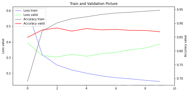
训练可视化

可以发现明显过拟合了

fig = plt.gcf()
fig.set_size_inches(10, 5)
ax1 = fig.add_subplot(111)
ax1.set_title('Train and Validation Picture')
ax1.set_ylabel('Loss value')
line1, = ax1.plot(history.history['loss'], color=(0.5, 0.5, 1.0), label='Loss train')
line2, = ax1.plot(history.history['val_loss'], color=(0.5, 1.0, 0.5), label='Loss valid')
ax2 = ax1.twinx()
ax2.set_ylabel('Accuracy value')
line3, = ax2.plot(history.history['accuracy'], color=(0.5, 0.5, 0.5), label='Accuracy train')
line4, = ax2.plot(history.history['val_accuracy'], color=(1, 0, 0), label='Accuracy valid')
plt.legend(handles=(line1, line2, line3, line4), loc='best')
plt.xlim(-1, 10)
plt.show()

准确率评估

我们发现利用已包装好的文件只能预测已包装好的文本，无法对现场摘取的文本进行预测，因为我们不知道其单词与数字的对应关系，在后面的 RNN(LSTM)我们将利用 TensorFlow1.x 手动处理数据集方式

test_loss, test_acc = model.evaluate(x_test, test_labels, verbose=2)
print('Test accuracy：', test_acc)

25000/1 - 3s - loss: 0.3215 - accuracy: 0.8564
Test accuracy： 0.85644

利用模型预测外部评论

选取星球大战中的一则评论:


《星球大战前传V-帝国反击战》于1980年上映，距今取得了巨大成功。要说《帝国反击战》向《新希望》伸张正义，那就是轻描淡写，因为这部电影以各种可能的方式提高了赌注。更长更好的战斗（例如完美无缺的霍斯之战），更黑暗，更成熟的情节，是有史以来最令人难忘（且被引用）的曲折之一，AT-AT步行者，Yoda的推出是一些原因为什么《帝国反击战》是完美的续集。与《新希望》不同，这部电影不是乔治·卢卡斯执导的，而是欧文·克什纳执导的，在他应得的荣誉中，他表现出色。克什纳（Kershner）还设法从演员阵容中获得最佳表现，尤其是哈米尔（Hamill），自上一部电影以来，他的性格发生了巨大变化。我们还看到了更多的维达及其疯狂而近乎动物的性格，詹姆斯·厄尔·琼斯的嗓音再次完美地展现了这一点。《帝国反击战》确实是完美的续集，因为它充实了乔治·卢卡斯的元素，并且大量继承了自己的作品。最终成绩-9 + / 10


中文翻译来源 Google Translate


可以看出这是一则好评

review_text='''Star Wars Episode V - The Empire Strikes Back was released in 1980, three years after its overwhelmingly successful predecessor.
        To say The Empire Strikes Back does justice to A New Hope is a massive understatement as this film ups the ante in every way possible. Longer and better battles (such as the immaculate Battle of Hoth), a much darker and more mature plot with one of the most memorable (and quoted) twists of all time, AT-AT walkers, the introduction of Yoda are some of the reasons why Empire Strikes Back is the perfect sequel.
        Unlike A New Hope, this film was not directed by George Lucas but Irvin Kershner and to give credit where credit is due he did just as good of a job. Kershner also manages to get the best possible performances out of his cast, especially Hamill whose character changed drastically since the last film. We also see more of Vader and his deranged and almost animalistic character which is again perfectly displayed by James Earl Jones's vocals.
        Empire Strikes Back truly is the perfect sequel as it flourishes on George Lucas's elements as well as bringing in many more of its own in great succession.
        Final Grade - 9+/10
      '''

text_to_list = tf.keras.preprocessing.text.text_to_word_sequence(
    review_text
)

word_index = imdb.get_word_index()
NUM_list = [word_index[key]+3 for key in text_to_list]
num_list = NUM_list.copy()

for i in range(len(num_list)):
    if num_list[i] >= 5000:
        num_list[i] = 2

test_list = tf.keras.preprocessing.sequence.pad_sequences([num_list],
                             padding='post',
                             truncating='post',
                             maxlen=length)

在 TensorFlow2.x 中，Imdb 数据集 1 代表 positive，0 代表 negtive，说明链接

sentiment_dict = {1:'pos', 0:'neg'}

pred = model.predict(test_list)
print('predict value:', sentiment_dict[np.argmax(pred)])

predict value: pos

文本还原

获取字典，注意需要输入原始数据集，而不是截长补短后的

word_index = imdb.get_word_index()
reverse_word_index = dict([(value, key) for (key, value) in word_index.items()])

review = [reverse_word_index.get(i-3, "?") for i in train_data[0]]

print('train_data[0] revert:\n', review)

train_data[0] revert:
 ['?', 'this', 'film', 'was', 'just', 'brilliant', 'casting', 'location', 'scenery', 'story', 'direction', "everyone's", 'really', 'suited', 'the', 'part', 'they', 'played', 'and', 'you', 'could', 'just', 'imagine', 'being', 'there', 'robert', '?', 'is', 'an', 'amazing', 'actor', 'and', 'now', 'the', 'same', 'being', 'director', '?', 'father', 'came', 'from', 'the', 'same', 'scottish', 'island', 'as', 'myself', 'so', 'i', 'loved', 'the', 'fact', 'there', 'was', 'a', 'real', 'connection', 'with', 'this', 'film', 'the', 'witty', 'remarks', 'throughout', 'the', 'film', 'were', 'great', 'it', 'was', 'just', 'brilliant', 'so', 'much', 'that', 'i', 'bought', 'the', 'film', 'as', 'soon', 'as', 'it', 'was', 'released', 'for', '?', 'and', 'would', 'recommend', 'it', 'to', 'everyone', 'to', 'watch', 'and', 'the', 'fly', '?', 'was', 'amazing', 'really', 'cried', 'at', 'the', 'end', 'it', 'was', 'so', 'sad', 'and', 'you', 'know', 'what', 'they', 'say', 'if', 'you', 'cry', 'at', 'a', 'film', 'it', 'must', 'have', 'been', 'good', 'and', 'this', 'definitely', 'was', 'also', '?', 'to', 'the', 'two', 'little', '?', 'that', 'played', 'the', '?', 'of', 'norman', 'and', 'paul', 'they', 'were', 'just', 'brilliant', 'children', 'are', 'often', 'left', 'out', 'of', 'the', '?', 'list', 'i', 'think', 'because', 'the', 'stars', 'that', 'play', 'them', 'all', 'grown', 'up', 'are', 'such', 'a', 'big', '?', 'for', 'the', 'whole', 'film', 'but', 'these', 'children', 'are', 'amazing', 'and', 'should', 'be', '?', 'for', 'what', 'they', 'have', 'done', "don't", 'you', 'think', 'the', 'whole', 'story', 'was', 'so', 'lovely', 'because', 'it', 'was', 'true', 'and', 'was', "someone's", 'life', 'after', 'all', 'that', 'was', '?', 'with', 'us', 'all']

train_data[0] 在 Imdb 数据集对应着 aclImdb/train/pos/576_10.txt 这个文件，读取这个文件并做对比

with open('./data/aclImdb/train/pos/576_10.txt', 'r') as file:
    message = file.readline()
    print(message)

this film was just brilliant,casting,location scenery,story,direction,everyone's really suited the part they played,and you could just imagine being there,Robert Redford's is an amazing actor and now the same being director,Norman's father came from the same Scottish island as myself,so i loved the fact there was a real connection with this film,the witty remarks throughout the film were great,it was just brilliant,so much that i bought the film as soon as it was released for retail and would recommend it to everyone to watch,and the fly-fishing was amazing,really cried at the end it was so sad,and you know what they say if you cry at a film it must have been good,and this definitely was, also congratulations to the two little boy's that played the part's of Norman and Paul they were just brilliant,children are often left out of the praising list i think, because the stars that play them all grown up are such a big profile for the whole film,but these children are amazing and should be praised for what they have done, don't you think? the whole story was so lovely because it was true and was someone's life after all that was shared with us all.

星球大战评论还原，使用未处理的 NUM_list

word_index = imdb.get_word_index()
reverse_word_index = dict([(value, key) for (key, value) in word_index.items()])

review = [reverse_word_index.get(i-3, "?") for i in NUM_list]

print('NUM_list revert:\n', review)

NUM_list revert:
 ['star', 'wars', 'episode', 'v', 'the', 'empire', 'strikes', 'back', 'was', 'released', 'in', '1980', 'three', 'years', 'after', 'its', 'overwhelmingly', 'successful', 'predecessor', 'to', 'say', 'the', 'empire', 'strikes', 'back', 'does', 'justice', 'to', 'a', 'new', 'hope', 'is', 'a', 'massive', 'understatement', 'as', 'this', 'film', 'ups', 'the', 'ante', 'in', 'every', 'way', 'possible', 'longer', 'and', 'better', 'battles', 'such', 'as', 'the', 'immaculate', 'battle', 'of', 'hoth', 'a', 'much', 'darker', 'and', 'more', 'mature', 'plot', 'with', 'one', 'of', 'the', 'most', 'memorable', 'and', 'quoted', 'twists', 'of', 'all', 'time', 'at', 'at', 'walkers', 'the', 'introduction', 'of', 'yoda', 'are', 'some', 'of', 'the', 'reasons', 'why', 'empire', 'strikes', 'back', 'is', 'the', 'perfect', 'sequel', 'unlike', 'a', 'new', 'hope', 'this', 'film', 'was', 'not', 'directed', 'by', 'george', 'lucas', 'but', 'irvin', 'kershner', 'and', 'to', 'give', 'credit', 'where', 'credit', 'is', 'due', 'he', 'did', 'just', 'as', 'good', 'of', 'a', 'job', 'kershner', 'also', 'manages', 'to', 'get', 'the', 'best', 'possible', 'performances', 'out', 'of', 'his', 'cast', 'especially', 'hamill', 'whose', 'character', 'changed', 'drastically', 'since', 'the', 'last', 'film', 'we', 'also', 'see', 'more', 'of', 'vader', 'and', 'his', 'deranged', 'and', 'almost', 'animalistic', 'character', 'which', 'is', 'again', 'perfectly', 'displayed', 'by', 'james', 'earl', "jones's", 'vocals', 'empire', 'strikes', 'back', 'truly', 'is', 'the', 'perfect', 'sequel', 'as', 'it', 'flourishes', 'on', 'george', "lucas's", 'elements', 'as', 'well', 'as', 'bringing', 'in', 'many', 'more', 'of', 'its', 'own', 'in', 'great', 'succession', 'final', 'grade', '9', '10']

思考

先看这几个参数(前面已有中文释义)
•skip_top: skip the top N most frequently occurring words (which may not be informative).
•start_char: The start of a sequence will be marked with this character. Set to 1 because 0 is usually the padding character.
•oov_char: words that were cut out because of the num_words or skip_top limit will be replaced with this character.

那么对星球大战评论预处理方式正确吗？其实是不正确的，虽然能够还原，但在处理时忽略了一些参数的设置，从
tf.keras.datasets.imdb.load_data(path=‘imdb.npz’, num_words=None, skip_top=0, maxlen=None, seed=113,
    start_char=1, oov_char=2, index_from=3, **kwargs)参数设置
与实际打印出的训练数据的值，可以发现，训练数据第一个数值都是 1，这是根据 start_char 参数设定的，在数字列表超过阈值（这里读取设定为 5000），将超过的值用 skip_top 与 oov_char 替换，甚至还有 index_from 参数，而我们仅仅将超过 5000 的阈值用 skip_top=0 代替，这不免与原始数据集有一些误差，但是 TensorFlow2.x 也未提供如何将新的文本转换为数字列表，所以也就只有将就了

RNN(LSTM)实现正式开始

导入必要包

import numpy as np
import datetime
import os
import re

必要函数定义

文件获取函数

def read_files(filetype):
    path = './data/aclImdb/'
    file_list = []

    positive_path = path + filetype + "/pos/"
    for f in os.listdir(positive_path):
        file_list += [positive_path + f]
    pos_files_num = len(file_list)

    negative_path = path + filetype + '/neg/'
    for f in os.listdir(negative_path):
        file_list += [negative_path + f]
    neg_files_num = len(file_list) - pos_files_num

    print('read', filetype, 'files:', len(file_list))
    print(pos_files_num, 'pos files in', filetype, 'files')
    print(neg_files_num, 'neg files in', filetype, 'files')

    all_labels = ([[1, 0]] * pos_files_num + [[0, 1]] * neg_files_num)
    all_texts = []
    for fi in file_list:
        with open(fi, encoding='utf8') as file_input:
            all_texts += [remove_tags(" ".join(file_input.readlines()))]

    return all_labels, all_texts

数据特殊字符处理(主要针对 html 残留格式)

def remove_tags(text):
    re_tag = re.compile(r'<[^>]+>')
    return re_tag.sub('', text)

train_labels, train_texts = read_files("train")
test_labels, test_texts = read_files("test")

read train files: 25000
12500 pos files in train files
12500 neg files in train files
read test files: 25000
12500 pos files in test files
12500 neg files in test files

print("训练数据，正面评价例子 文本：", train_texts[0])
print("训练数据，正面评价例子 标签：", train_labels[0])
print("训练数据，负面评价例子 文本：", train_texts[12500])
print("训练数据，负面评价例子 标签：", train_labels[12500])

print("测试数据，正面评价例子 文本：", test_texts[0])
print("测试数据，正面评价例子 标签：", test_labels[0])
print("测试数据，负面评价例子 文本：", test_texts[12500])
print("测试数据，负面评价例子 标签：", test_labels[12500])

训练数据，正面评价例子 文本： Bromwell High is a cartoon comedy. It ran at the same time as some other programs about school life, such as "Teachers". My 35 years in the teaching profession lead me to believe that Bromwell High's satire is much closer to reality than is "Teachers". The scramble to survive financially, the insightful students who can see right through their pathetic teachers' pomp, the pettiness of the whole situation, all remind me of the schools I knew and their students. When I saw the episode in which a student repeatedly tried to burn down the school, I immediately recalled ......... at .......... High. A classic line: INSPECTOR: I'm here to sack one of your teachers. STUDENT: Welcome to Bromwell High. I expect that many adults of my age think that Bromwell High is far fetched. What a pity that it isn't!
训练数据，正面评价例子 标签： [1, 0]
训练数据，负面评价例子 文本： Story of a man who has unnatural feelings for a pig. Starts out with a opening scene that is a terrific example of absurd comedy. A formal orchestra audience is turned into an insane, violent mob by the crazy chantings of it's singers. Unfortunately it stays absurd the WHOLE time with no general narrative eventually making it just too off putting. Even those from the era should be turned off. The cryptic dialogue would make Shakespeare seem easy to a third grader. On a technical level it's better than you might think with some good cinematography by future great Vilmos Zsigmond. Future stars Sally Kirkland and Frederic Forrest can be seen briefly.
训练数据，负面评价例子 标签： [0, 1]
测试数据，正面评价例子 文本： I went and saw this movie last night after being coaxed to by a few friends of mine. I'll admit that I was reluctant to see it because from what I knew of Ashton Kutcher he was only able to do comedy. I was wrong. Kutcher played the character of Jake Fischer very well, and Kevin Costner played Ben Randall with such professionalism. The sign of a good movie is that it can toy with our emotions. This one did exactly that. The entire theater (which was sold out) was overcome by laughter during the first half of the movie, and were moved to tears during the second half. While exiting the theater I not only saw many women in tears, but many full grown men as well, trying desperately not to let anyone see them crying. This movie was great, and I suggest that you go see it before you judge.
测试数据，正面评价例子 标签： [1, 0]
测试数据，负面评价例子 文本： Once again Mr. Costner has dragged out a movie for far longer than necessary. Aside from the terrific sea rescue sequences, of which there are very few I just did not care about any of the characters. Most of us have ghosts in the closet, and Costner's character are realized early on, and then forgotten until much later, by which time I did not care. The character we should really care about is a very cocky, overconfident Ashton Kutcher. The problem is he comes off as kid who thinks he's better than anyone else around him and shows no signs of a cluttered closet. His only obstacle appears to be winning over Costner. Finally when we are well past the half way point of this stinker, Costner tells us all about Kutcher's ghosts. We are told why Kutcher is driven to be the best with no prior inkling or foreshadowing. No magic here, it was all I could do to keep from turning it off an hour in.
测试数据，负面评价例子 标签： [0, 1]

建立词汇词典

token = tf.keras.preprocessing.text.Tokenizer(num_words=5000)

token.fit_on_texts(train_texts)

查看读取文档数

print('Files read', token.document_count)

Files read 25000

注意以下三个 print 输出太长，运行结果未写入博客
单词映射排名或索引

print('Word index', token.word_index)

单词映射为训练期间所出现文档或文本数量

print(token.word_docs)

获取各词出现频率

print(token.word_counts)

文字转数字列表

train_sequences = token.texts_to_sequences(train_texts)
test_sequences = token.texts_to_sequences(test_texts)

print("文本信息：\n", train_texts[0])
print("对应数字信息：\n", train_sequences[0])

文本信息：
 Bromwell High is a cartoon comedy. It ran at the same time as some other programs about school life, such as "Teachers". My 35 years in the teaching profession lead me to believe that Bromwell High's satire is much closer to reality than is "Teachers". The scramble to survive financially, the insightful students who can see right through their pathetic teachers' pomp, the pettiness of the whole situation, all remind me of the schools I knew and their students. When I saw the episode in which a student repeatedly tried to burn down the school, I immediately recalled ......... at .......... High. A classic line: INSPECTOR: I'm here to sack one of your teachers. STUDENT: Welcome to Bromwell High. I expect that many adults of my age think that Bromwell High is far fetched. What a pity that it isn't!
对应数字信息：
 [308, 6, 3, 1068, 208, 8, 2160, 29, 1, 168, 54, 13, 45, 81, 40, 391, 109, 137, 13, 57, 4445, 149, 7, 1, 4986, 481, 68, 5, 260, 11, 2000, 6, 72, 2422, 5, 631, 70, 6, 1, 5, 2001, 1, 1530, 33, 66, 63, 204, 139, 64, 1229, 1, 4, 1, 222, 899, 28, 3021, 68, 4, 1, 9, 693, 2, 64, 1530, 50, 9, 215, 1, 386, 7, 59, 3, 1470, 3710, 798, 5, 3509, 176, 1, 391, 9, 1235, 29, 308, 3, 352, 343, 2970, 142, 129, 5, 27, 4, 125, 1470, 2372, 5, 308, 9, 532, 11, 107, 1466, 4, 57, 554, 100, 11, 308, 6, 226, 4173, 47, 3, 2231, 11, 8, 214]

文本截长补短

以 300 为例

x_train = tf.keras.preprocessing.sequence.pad_sequences(train_sequences,
                             padding='post',
                             truncating='post',
                             maxlen=300)
x_test = tf.keras.preprocessing.sequence.pad_sequences(test_sequences,
                             padding='post',
                             truncating='post',
                             maxlen=300)

x_train.shape

(25000, 300)

y_train = np.array(train_labels)
y_test = np.array(test_labels)

print("填充后数字列表：\n", x_train[0])

填充后数字列表：
 [ 308    6    3 1068  208    8 2160   29    1  168   54   13   45   81
   40  391  109  137   13   57 4445  149    7    1 4986  481   68    5
  260   11 2000    6   72 2422    5  631   70    6    1    5 2001    1
 1530   33   66   63  204  139   64 1229    1    4    1  222  899   28
 3021   68    4    1    9  693    2   64 1530   50    9  215    1  386
    7   59    3 1470 3710  798    5 3509  176    1  391    9 1235   29
  308    3  352  343 2970  142  129    5   27    4  125 1470 2372    5
  308    9  532   11  107 1466    4   57  554  100   11  308    6  226
 4173   47    3 2231   11    8  214    0    0    0    0    0    0    0
    0    0    0    0    0    0    0    0    0    0    0    0    0    0
    0    0    0    0    0    0    0    0    0    0    0    0    0    0
    0    0    0    0    0    0    0    0    0    0    0    0    0    0
    0    0    0    0    0    0    0    0    0    0    0    0    0    0
    0    0    0    0    0    0    0    0    0    0    0    0    0    0
    0    0    0    0    0    0    0    0    0    0    0    0    0    0
    0    0    0    0    0    0    0    0    0    0    0    0    0    0
    0    0    0    0    0    0    0    0    0    0    0    0    0    0
    0    0    0    0    0    0    0    0    0    0    0    0    0    0
    0    0    0    0    0    0    0    0    0    0    0    0    0    0
    0    0    0    0    0    0    0    0    0    0    0    0    0    0
    0    0    0    0    0    0    0    0    0    0    0    0    0    0
    0    0    0    0    0    0]

模型构建

model = tf.keras.models.Sequential()

在前一篇博客中有tf.keras.layers.GlobalAveragePooling2D()代替全连接层，全局池化在神经网络的全连接层具有一定的优越性，上面已使用一次，这里使用tf.keras.layers.Flatten()

model.add(tf.keras.layers.Embedding(output_dim=32,
                  input_dim=5000,
                  input_length=300))

model.add(tf.keras.layers.Flatten())
model.add(tf.keras.layers.Dense(units=256, activation='relu'))
model.add(tf.keras.layers.Dropout(0.3))
model.add(tf.keras.layers.Dense(units=2, activation='softmax'))

model.summary()

Model: "sequential_1"
_________________________________________________________________
Layer (type)                 Output Shape              Param #   
=================================================================
embedding_1 (Embedding)      (None, 300, 32)           160000    
_________________________________________________________________
flatten (Flatten)            (None, 9600)              0         
_________________________________________________________________
dense_2 (Dense)              (None, 256)               2457856   
_________________________________________________________________
dropout_1 (Dropout)          (None, 256)               0         
_________________________________________________________________
dense_3 (Dense)              (None, 2)                 514       
=================================================================
Total params: 2,618,370
Trainable params: 2,618,370
Non-trainable params: 0
_________________________________________________________________

model.compile(optimizer='adam',
       loss='categorical_crossentropy',
       metrics=['accuracy'])

log_dir = os.path.join(
    'logs2.x',
    'train',
    'plugins',
    'profile',
    datetime.datetime.now().strftime('%Y-%m-%d_%H-%M-%S'))

checkpoint_path = './checkpoint2.x/nlp.{epoch:02d}.h5'

if not os.path.exists('./checkpoint2.x'):
    os.mkdir('./checkpoint2.x')


callbacks = [
    tf.keras.callbacks.TensorBoard(log_dir=log_dir,
                         histogram_freq=2),
    tf.keras.callbacks.ModelCheckpoint(filepath=checkpoint_path,
                                       save_weights_only=True,
                                       verbose=0,
                                       save_freq='epoch'),
    tf.keras.callbacks.EarlyStopping(monitor='val_accuracy', patience=5)
]

history = model.fit(x_train,
            y_train,
            validation_split=0.2,
            epochs=20,
            batch_size=128,
            callbacks=callbacks,
            verbose=1)

Train on 20000 samples, validate on 5000 samples
Epoch 1/20
20000/20000 [==============================] - 3s 147us/sample - loss: 5.4748e-04 - accuracy: 1.0000 - val_loss: 1.2081 - val_accuracy: 0.7682
Epoch 2/20
20000/20000 [==============================] - 3s 130us/sample - loss: 3.3104e-04 - accuracy: 1.0000 - val_loss: 1.1862 - val_accuracy: 0.7804
Epoch 3/20
20000/20000 [==============================] - 3s 142us/sample - loss: 2.4753e-04 - accuracy: 1.0000 - val_loss: 1.2905 - val_accuracy: 0.7690
Epoch 4/20
20000/20000 [==============================] - 3s 138us/sample - loss: 1.7880e-04 - accuracy: 1.0000 - val_loss: 1.2901 - val_accuracy: 0.7726
Epoch 5/20
20000/20000 [==============================] - 3s 151us/sample - loss: 1.3524e-04 - accuracy: 1.0000 - val_loss: 1.3295 - val_accuracy: 0.7720
Epoch 6/20
20000/20000 [==============================] - 3s 130us/sample - loss: 1.0861e-04 - accuracy: 1.0000 - val_loss: 1.3143 - val_accuracy: 0.7790
Epoch 7/20
20000/20000 [==============================] - 3s 140us/sample - loss: 9.1809e-05 - accuracy: 1.0000 - val_loss: 1.3301 - val_accuracy: 0.7800

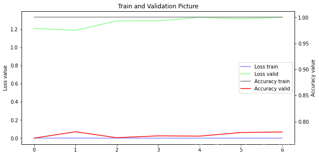
训练可视乎

由于加入了监控 val_accuracy 的早停参数，训练 7 轮截至

fig = plt.gcf()
fig.set_size_inches(10, 5)
ax1 = fig.add_subplot(111)
ax1.set_title('Train and Validation Picture')
ax1.set_ylabel('Loss value')
line1, = ax1.plot(history.history['loss'], color=(0.5, 0.5, 1.0), label='Loss train')
line2, = ax1.plot(history.history['val_loss'], color=(0.5, 1.0, 0.5), label='Loss valid')
ax2 = ax1.twinx()
ax2.set_ylabel('Accuracy value')
line3, = ax2.plot(history.history['accuracy'], color=(0.5, 0.5, 0.5), label='Accuracy train')
line4, = ax2.plot(history.history['val_accuracy'], color=(1, 0, 0), label='Accuracy valid')
plt.legend(handles=(line1, line2, line3, line4), loc='best')
plt.show()

模型评估

test_loss, test_acc = model.evaluate(x_test, y_test, verbose=2)
print('Test accuracy：', test_acc)

25000/1 - 8s - loss: 2.1999 - accuracy: 0.8380
Test accuracy： 0.83804

利用模型预测外部评论

review_text='''Star Wars Episode V - The Empire Strikes Back was released in 1980, three years after its overwhelmingly successful predecessor.
        To say The Empire Strikes Back does justice to A New Hope is a massive understatement as this film ups the ante in every way possible. Longer and better battles (such as the immaculate Battle of Hoth), a much darker and more mature plot with one of the most memorable (and quoted) twists of all time, AT-AT walkers, the introduction of Yoda are some of the reasons why Empire Strikes Back is the perfect sequel.
        Unlike A New Hope, this film was not directed by George Lucas but Irvin Kershner and to give credit where credit is due he did just as good of a job. Kershner also manages to get the best possible performances out of his cast, especially Hamill whose character changed drastically since the last film. We also see more of Vader and his deranged and almost animalistic character which is again perfectly displayed by James Earl Jones's vocals.
        Empire Strikes Back truly is the perfect sequel as it flourishes on George Lucas's elements as well as bringing in many more of its own in great succession.
        Final Grade - 9+/10
      '''

sentiment_dict = {0:'pos', 1:'neg'}

def display_text_sentiment(text):
    print(text)
    input_seq = token.texts_to_sequences([text])
    pad_input_seq = tf.keras.preprocessing.sequence.pad_sequences(input_seq,
                                  padding='post',
                                  truncating='post',
                                  maxlen=300)
    pred = model.predict(pad_input_seq)
    print('predict value:', sentiment_dict[np.argmax(pred)])

display_text_sentiment(review_text)

Star Wars Episode V - The Empire Strikes Back was released in 1980, three years after its overwhelmingly successful predecessor.
        To say The Empire Strikes Back does justice to A New Hope is a massive understatement as this film ups the ante in every way possible. Longer and better battles (such as the immaculate Battle of Hoth), a much darker and more mature plot with one of the most memorable (and quoted) twists of all time, AT-AT walkers, the introduction of Yoda are some of the reasons why Empire Strikes Back is the perfect sequel.
        Unlike A New Hope, this film was not directed by George Lucas but Irvin Kershner and to give credit where credit is due he did just as good of a job. Kershner also manages to get the best possible performances out of his cast, especially Hamill whose character changed drastically since the last film. We also see more of Vader and his deranged and almost animalistic character which is again perfectly displayed by James Earl Jones's vocals.
        Empire Strikes Back truly is the perfect sequel as it flourishes on George Lucas's elements as well as bringing in many more of its own in great succession.
        Final Grade - 9+/10
      
predict value: pos

导入已存储模型进行识别

注意tf.train.latest_checkpoint只适用于ckpt形式

model.load_weights('./checkpoint2.x/nlp.07.h5')

display_text_sentiment(review_text)

Star Wars Episode V - The Empire Strikes Back was released in 1980, three years after its overwhelmingly successful predecessor.
        To say The Empire Strikes Back does justice to A New Hope is a massive understatement as this film ups the ante in every way possible. Longer and better battles (such as the immaculate Battle of Hoth), a much darker and more mature plot with one of the most memorable (and quoted) twists of all time, AT-AT walkers, the introduction of Yoda are some of the reasons why Empire Strikes Back is the perfect sequel.
        Unlike A New Hope, this film was not directed by George Lucas but Irvin Kershner and to give credit where credit is due he did just as good of a job. Kershner also manages to get the best possible performances out of his cast, especially Hamill whose character changed drastically since the last film. We also see more of Vader and his deranged and almost animalistic character which is again perfectly displayed by James Earl Jones's vocals.
        Empire Strikes Back truly is the perfect sequel as it flourishes on George Lucas's elements as well as bringing in many more of its own in great succession.
        Final Grade - 9+/10
      
predict value: pos