from keras.datasets import imdb
#num_words表示加载影评时,确保影评里面的单词使用频率保持在前1万位,于是有些很少见的生僻词在数据加载时会舍弃掉
(train_data, train_labels), (test_data, test_labels) = imdb.load_data(num_words=10000)
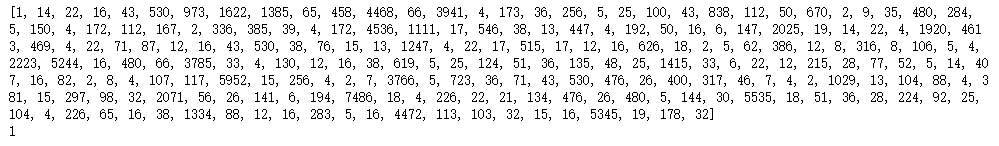
print(train_data[0])
print(train_labels[0])
#频率与单词的对应关系存储在哈希表word_index中,它的key对应的是单词,value对应的是单词的频率
word_index = imdb.get_word_index()
#我们要把表中的对应关系反转一下,变成key是频率,value是单词
reverse_word_index = dict([(value, key) for (key, value) in word_index.items()])
'''
在train_data所包含的数值中,数值1,2,3对应的不是单词,而用来表示特殊含义,1表示“填充”,2表示”文本起始“,
3表示”未知“,因此当我们从train_data中读到的数值是1,2,3时,我们要忽略它,从4开始才对应单词,如果数值是4,
那么它表示频率出现最高的单词
'''
text = ""
for wordCount in train_data[0]:
    if wordCount > 3:
        text += reverse_word_index.get(wordCount - 3)
        text += " "
    else:
        text += "?"

print(text)

import numpy as np
def oneHotVectorizeText(allText, dimension=10000):
    '''
    allText是所有文本集合,每条文本对应一个含有10000个元素的一维向量,假设文本总共有X条,那么
    该函数会产生X条维度为一万的向量,于是形成一个含有X行10000列的二维矩阵
    '''
    oneHotMatrix = np.zeros((len(allText), dimension))
    for i, wordFrequence in enumerate(allText):
        oneHotMatrix[i, wordFrequence] = 1.0
    return oneHotMatrix

x_train = oneHotVectorizeText(train_data)
x_test =  oneHotVectorizeText(test_data)

print(x_train[0])

y_train = np.asarray(train_labels).astype('float32')
y_test = np.asarray(test_labels).astype('float32')
from keras import models
from keras import layers
model = models.Sequential()
#构建第一层和第二层网络,第一层有10000个节点,第二层有16个节点
#Dense的意思是,第一层每个节点都与第二层的所有节点相连接
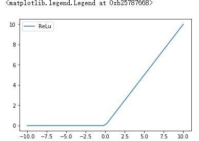
#relu 对应的函数是relu(x) = max(0, x)
model.add(layers.Dense(16, activation='relu', input_shape=(10000,)))
#第三层有16个神经元,第二层每个节点与第三层每个节点都相互连接
model.add(layers.Dense(16, activation='relu'))
#第四层只有一个节点,输出一个0-1之间的概率值
model.add(layers.Dense(1, activation='sigmoid'))
import matplotlib.pyplot as plt
x = np.linspace(-10, 10)
y_relu = np.array([0*item if item < 0 else item for item in x])
plt.figure()
plt.plot(x, y_relu, label='ReLu')
plt.legend()
from keras import losses
from keras import metrics
from keras import optimizers

model.compile(optimizer=optimizers.RMSprop(lr=0.001), loss='binary_crossentropy', metrics=['accuracy'])
x_val = x_train[:10000]
partial_x_train = x_train[10000:]
y_val = y_train[: 10000]
partial_y_train = y_train[10000:]
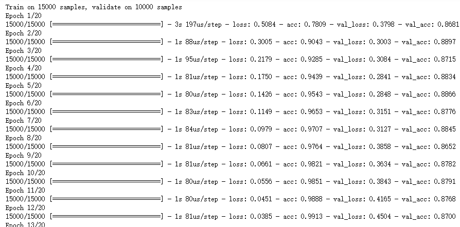
history = model.fit(partial_x_train, partial_y_train, epochs=20, batch_size=512,
validation_data = (x_val, y_val))
train_result = history.history
print(train_result.keys())

import matplotlib.pyplot as plt
acc = train_result['acc']
val_acc = train_result['val_acc']
loss = train_result['loss']
val_loss = train_result['val_loss']
epochs = range(1, len(acc) + 1)
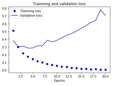
#绘制训练数据识别准确度曲线
plt.plot(epochs, loss, 'bo', label='Trainning loss')
#绘制校验数据识别的准确度曲线
plt.plot(epochs, val_loss, 'b', label='Validation loss')
plt.title('Trainning and validation loss')
plt.xlabel('Epochs')
plt.ylabel('Loss')
plt.legend()
plt.show()
model = models.Sequential()
model.add(layers.Dense(16, activation='relu', input_shape=(10000,)))
model.add(layers.Dense(16, activation='relu'))
model.add(layers.Dense(1, activation='sigmoid'))
model.compile(optimizer='rmsprop',
loss='binary_crossentropy',
metrics=['accuracy'])
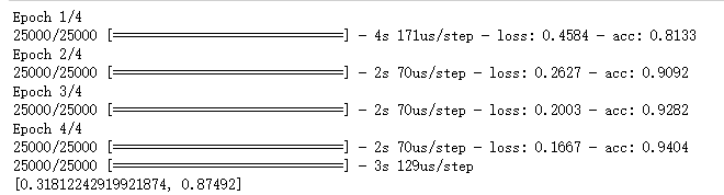
history = model.fit(x_train, y_train, epochs=4, batch_size=512)
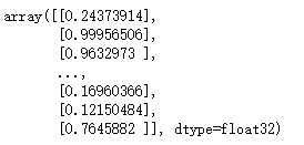
results = model.evaluate(x_test, y_test)
print(results)