数据挖掘基础知识储备——Pandas

Python之所以对处理数据非常方便，不得不说Numpy与Pdndas功不可没～
本篇博客将总结所有关于数据挖掘中常用到的pandas的使用方法，阅读好的代码往往有利于代码的书写和方便他人阅读，这是一个很好的习惯呀～
推荐Pandas中文官方文档：Click～

数据结构

维数	名称	描述
1	Series	带标签的一维同构数组
2	DataFrame	带标签的，大小可变的，二维异构表格

导库

import numpy as np
import pandas as pd

#设置这个在数据非常多的时候会更直观
pd.set_option('display.max_columns', None)
pd.set_option('display.max_rows', None)

基本操作

构造一个DataFrame

df = pd.DataFrame({'A': 1.,
   ...:            'B': pd.Timestamp('20130102'),
   ...:            'C': pd.Series(1, index=list(range(4)), dtype='float32'),
   ...:            'D': np.array([3] * 4, dtype='int32'),
   ...:            'E': pd.Categorical(["test", "train", "test", "train"]),
   ...:            'F': 'foo',
   ...:            'G': pd.Series(i*6%7 for i in range(4))})

#可以直接生成一个复制品
df2 = df.copy()

查看

输出DataFrame

df

	A	B	C	D	E	F	G
0	1.0	2013-01-02	1.0	3	test	foo	0
1	1.0	2013-01-02	1.0	3	train	foo	6
2	1.0	2013-01-02	1.0	3	test	foo	5
3	1.0	2013-01-02	1.0	3	train	foo	4

查看数据类型

df.dtypes

A           float64
B    datetime64[ns]
C           float32
D             int32
E          category
F            object
G             int64
dtype: object

查看前几行数据

df.head(2)

查看后两行数据

df.tail(3)

查看数据统计情况

df.describe()

查看行标

df.index

Int64Index([0, 1, 2, 3], dtype='int64')

查看列标

df.columns

Index(['A', 'B', 'C', 'D', 'E', 'F', 'G'], dtype='object')

查看某列数据

df['A']

df.A

排序

对标签进行排序

# 参数axis=0说明按行标签排序，asix=1说明按列标签排序，ascend==True开启升序排序
df.sort_index(axis=0, ascending=False)

df.sort_index(axis=1, ascending=False)

对某列进行排序

df.sort_values(by='B')

选择

按标签选择

通过上面的index和columns的取值和类型：loc

df.loc[:,['A','B']]

	A	B
0	1.0	2013-01-02
1	1.0	2013-01-02
2	1.0	2013-01-02
3	1.0	2013-01-02

df.loc[[1,2],:]

	A	B	C	D	E	F	G
0	1.0	2013-01-02	1.0	3	test	foo	0
1	1.0	2013-01-02	1.0	3	train	foo	6

按位置选择

数字表示第几行第几列，从0开始：iloc

df.iloc[:,3]

#表示取第四列
0    3
1    3
2    3
3    3
Name: D, dtype: int32

df.iloc[3]

#表示第四行，pd取出来的某行或某列都是用一个序列serie s进行表示的
A                      1
B    2013-01-02 00:00:00
C                      1
D                      3
E                  train
F                    foo
G                      4
Name: 3, dtype: object

按条件选择

在框内指定条件

df[df.G>4]

	A	B	C	D	E	F	G
1	1.0	2013-01-02	1.0	3	train	foo	6
2	1.0	2013-01-02	1.0	3	test	foo	5

df[df.G.isin([0,4,8])]

	A	B	C	D	E	F	G
0	1.0	2013-01-02	1.0	3	test	foo	0
3	1.0	2013-01-02	1.0	3	train	foo	4

赋值

添加新标签，并且赋值

s1 = pd.Series([1, 2, 3, 4], index=range(4))
#添加新标签，并且赋值
df['H'] = s1

	A	B	C	D	E	F	G	H
0	1.0	2013-01-02	1.0	3	test	foo	0	1
1	1.0	2013-01-02	1.0	3	train	foo	6	2
2	1.0	2013-01-02	1.0	3	test	foo	5	3
3	1.0	2013-01-02	1.0	3	train	foo	4	4

按标签赋值

df.at[0, 'A'] = 0

	A	B	C	D	E	F	G	H
0	0.0	2013-01-02	1.0	3	test	foo	0	1
1	1.0	2013-01-02	1.0	3	train	foo	6	2
2	1.0	2013-01-02	1.0	3	test	foo	5	3
3	1.0	2013-01-02	1.0	3	train	foo	4	4

按位置赋值

df.iat[0, 3] = 5

	A	B	C	D	E	F	G	H
0	0.0	2013-01-02	1.0	5	test	foo	0	1
1	1.0	2013-01-02	1.0	3	train	foo	6	2
2	1.0	2013-01-02	1.0	3	test	foo	5	3
3	1.0	2013-01-02	1.0	3	train	foo	4	4

按 NumPy 数组赋值

df.loc[:,'D']=np.array([5]*len(df))

	A	B	C	D	E	F	G	H
0	0.0	2013-01-02	1.0	5	test	foo	0	1
1	1.0	2013-01-02	1.0	5	train	foo	6	2
2	1.0	2013-01-02	1.0	5	test	foo	5	3
3	1.0	2013-01-02	1.0	5	train	foo	4	4

用 where 条件赋值

df2 = df['G'].copy()
df2[df2>0]=-df2
df['G']=df2

	A	B	C	D	E	F	G	H
0	0.0	2013-01-02	1.0	5	test	foo	0	1
1	1.0	2013-01-02	1.0	5	train	foo	-6	2
2	1.0	2013-01-02	1.0	5	test	foo	-5	3
3	1.0	2013-01-02	1.0	5	train	foo	-4	4

缺失值

Pandas 主要用 np.nan 表示缺失数据。 计算时，默认不包含空值。
以下操作返回副本，不会在原DataFrame上进行修改，可以使用赋值对原本进行修改。

重建索引（reindex）

可以更改、添加、删除指定轴的索引，并返回数据副本，即不更改原数据。

df1 = df.iloc[:,0:3]
df1 = df1.reindex(index=range(4), columns=list(df1.columns) + ['D'])
df1.loc[0:1, 'D'] = 1

	A	B	C	D
0	0.0	2013-01-02	1.0	1.0
1	1.0	2013-01-02	1.0	1.0
2	1.0	2013-01-02	1.0	NaN
3	1.0	2013-01-02	1.0	NaN

删除所有含缺失值的行

df1.dropna(how='any')

	A	B	C	D
0	0.0	2013-01-02	1.0	1.0
1	1.0	2013-01-02	1.0	1.0

填充缺失值

df1.fillna(value=5)

	A	B	C	D
0	0.0	2013-01-02	1.0	1.0
1	1.0	2013-01-02	1.0	1.0
2	1.0	2013-01-02	1.0	5.0
3	1.0	2013-01-02	1.0	5.0

提取 nan 值的布尔掩码

pd.isna(df1)

	A	B	C	D
0	False	False	False	False
1	False	False	False	False
2	False	False	False	True
3	False	False	False	True

运算

df = pd.DataFrame(np.random.randn(3, 4),columns=['A','B','C','D'])

	A	B	C	D
0	-2.717438	0.945965	0.748211	1.245315
1	1.109978	-0.272390	0.628783	-0.226674
2	-0.818794	0.593518	-1.447567	-0.535336

统计

自带函数，有一系列相对应的函数啦
求平均数

df.mean()

A   -0.808751
B    0.422364
C   -0.023524
D    0.161102
dtype: float64

# 上面的是在列上的操作，这个是在行上的操作
df.mean(1)

0    0.055513
1    0.309924
2   -0.552045
dtype: float64

求众数

df.median()

A   -0.818794
B    0.593518
C    0.628783
D   -0.226674
dtype: float64

Apply 函数

Apply 函数处理数据

"""
apply以每列为单位，里面装一个函数
numpy.cumsum(a, axis=None, dtype=None, out=None)
axis=0，按照行累加。
axis=1，按照列累加。
"""
df.apply(np.cumsum)

	A	B	C	D
0	-2.717438	0.945965	0.748211	1.245315
1	-1.607460	0.673574	1.376994	1.018642
2	-2.426254	1.267092	-0.070573	0.483306

# apply以每列为单位，lambda执行一个匿名函数
df.apply(lambda x: x.max() - x.min())

A    3.827415
B    1.218355
C    2.195778
D    1.780651
dtype: float64

df.apply(lambda x:x*2)

	A	B	C	D
0	-5.434875	1.891929	1.496422	2.490630
1	2.219956	-0.544781	1.257565	-0.453347
2	-1.637588	1.187036	-2.895134	-1.070672

合并

结合Concat

df = pd.DataFrame(np.random.randn(10, 4))

#分解为多组
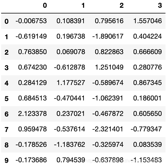
pieces = [df[:3], df[3:7], df[7:]]

pd.concat(pieces)

连接Join

风格和数据库的连接一样

left = pd.DataFrame({'key': ['foo', 'foo'], 'lval': [1, 2]})

	key	lval
0	foo	1
1	foo	2

right = pd.DataFrame({'key': ['foo', 'foo'], 'rval': [4, 5]})

	key	lval
0	foo	4
1	foo	5

pd.merge(left, right, on='key')

	key	lval	rval
0	foo	1	4
1	foo	1	5
2	foo	2	4
3	foo	2	5

追加Append

为 DataFrame 追加行

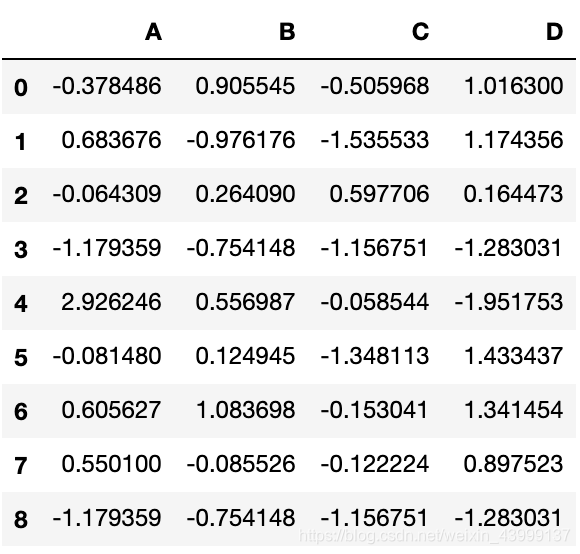
df = pd.DataFrame(np.random.randn(8, 4), columns=['A', 'B', 'C', 'D'])
s = df.iloc[3]
df.append(s, ignore_index=True)

分组（Grouping）

数据库经典操作
“group by” 指的是涵盖下列一项或多项步骤的处理流程：

• 分割：按条件把数据分割成多组；
• 应用：为每组单独应用函数；
• 组合：将处理结果组合成一个数据结构。

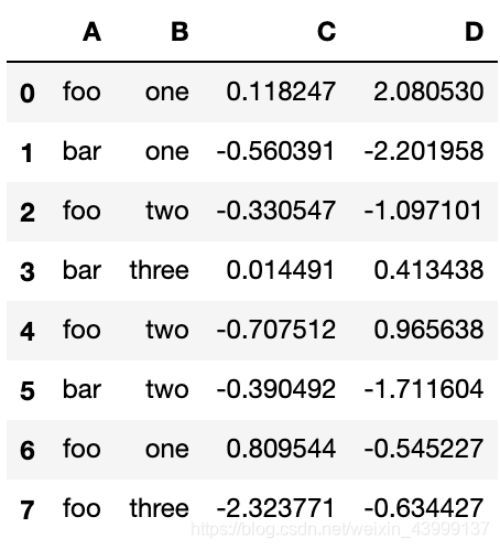
df = pd.DataFrame({'A': ['foo', 'bar', 'foo', 'bar',
   ....:                          'foo', 'bar', 'foo', 'foo'],
   ....:                    'B': ['one', 'one', 'two', 'three',
   ....:                          'two', 'two', 'one', 'three'],
   ....:                    'C': np.random.randn(8),
   ....:                    'D': np.random.randn(8)})

df.groupby('A').sum()

	C	D
A
bar	-0.936392	-3.500124
foo	-2.434039	0.769412

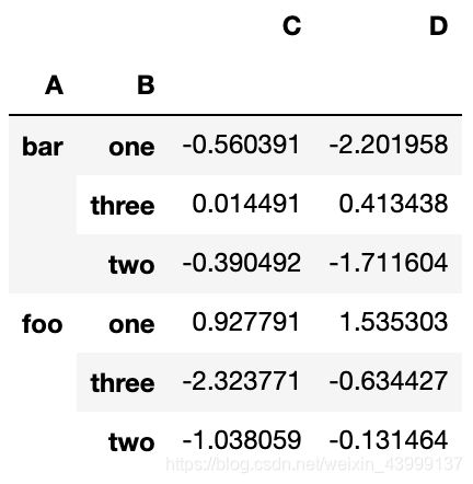
df.groupby(['A','B']).sum()

#分组后添加聚集函数噢噢，奥力给。和前面的效果是一样的
df.groupby(['A','B']).agg('sum')

总结

后面有坑在补，预计后期会补充一份数据挖掘中用到关于pandas的常见操作，和可视化库的学习啦～