二维函数求解最大值算法
- 1. 不同的求解算法:
对于二维函数求解最大值的算法,主要可以分为两大类,经过测试,各自算法的特点如下所示:
(1) 爬山算法
① 原理:假定所求问题有多个参数,我们在通过爬山法逐步获得最优解的过程中可以依次分别将某个参数的值增加或者减少一个单位。例如某个问题的解需要使用2个整数类型的参数x1、x2,开始时将这三个参数设值为(2,2),将x1增加/减少1,得到两个解(1,2), (3,2);将x2增加/减少1,得到两个解(2,3),(2,1),这样就得到了一个解集:
(2,2), (1, 2), (3, 2), (2,3), (2,1), (2,1), (2,2),从上面的解集中找到最优解,然后将这个最优解依据上面的方法再构造一个解集,再求最优解,就这样,直到前一次的最优解和后一次的最优解相同才结束“爬山”。
② 特点:思路比较简单,但是在求解当中,对于一些复杂的二维函数,容易收敛到局部最优解,对于一些简单的函数和约束区间,爬山算法也可以找到全局最优解;另外,爬山法比较适用于一元函数,其本质是梯度上升法。
(2) 遗传算法(或者粒子群算法):基于随机梯度变化,寻找一定区间里的最优解,原理比较复杂,可以对大多数情况找到二维函数的全局最优解,不太容易收敛到局部最优解。
基于以上的特点,可以采用两种算法相互辅助和检查的方法来进行计算全局最优解
2.二元函数求最大值算法实现(python版本):可直接使用
(1)爬山算法代码实现:
import random
#定义二维的函数表达式
def evaluate(x, y):
return -1*(x-1)**2+x*y+2*x
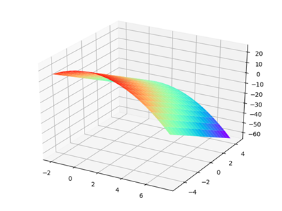
#画出二维函数的三维图像如下(可以用来检验求得解的合理性)
from mpl_toolkits.mplot3d import Axes3D
import numpy as np
from matplotlib import pyplot as plt
fig = plt.figure() #定义新的三维坐标轴
ax3 = plt.axes(projection='3d')
#定义三维数据
x = np.arange(-2,8,0.5)
y = np.arange(-5,5,0.5)
X, Y = np.meshgrid(x, y)
Z = -1*(X-1)**2+Y*X+2*X
ax3.plot_surface(X,Y,Z,cmap='rainbow')
plt.show()
#定义x和y的区间大小
x_range = [[-2, 8], [-5, 5]]
best_sol = [(x_range[0][0]),(x_range[1][0])]
while True:
best_evaluate = evaluate(best_sol[0], best_sol[1])
current_best_value = best_evaluate
sols = [best_sol]
for i in range(len(best_sol)):
if best_sol[i] > x_range[i][0]:
#设置变化的步长为0.01
sols.append(best_sol[0:i] + [best_sol[i]-0.01] + best_sol[i+1:])
if best_sol[i] < x_range[i][1]:
sols.append(best_sol[0:i] + [best_sol[i]+0.01] + best_sol[i+1:])
print(sols)
for s in sols:
el = evaluate(s[0], s[1])
if el > best_evaluate:
best_sol = s
best_evaluate = el
if best_evaluate == current_best_value:
break
#输出最优解和取得最优解时的x和y的取值大小
print('best sol:', current_best_value, best_sol)
(2)遗传算法源代码(较为复杂)
import numpy as np
import random
import math
import copy
class Ind():
def __init__(self):
self.fitness = 0
self.x = np.zeros(33)
self.place = 0
self.x1 = 0
self.x2 = 0
def Cal_fit(x, upper, lower): #计算适应度值函数
Temp1 = 0
for i in range(18):
Temp1 += x[i] * math.pow(2, i)
Temp2 = 0
for i in range(18, 33, 1):
Temp2 += math.pow(2, i - 18) * x[i]
x1 = lower[0] + Temp1 * (upper[0] - lower[0])/(math.pow(2, 18) - 1)
x2 = lower[1] + Temp2 * (upper[1] - lower[1])/(math.pow(2, 15) - 1)
if x1 > upper[0]:
x1 = random.uniform(lower[0], upper[0])
if x2 > upper[1]:
x2 = random.uniform(lower[1], upper[1])
#二维函数的具体表达形式
return -1*(x1-1)**2+x1*x2+2*x1
def Init(G, upper, lower, Pop): #初始化函数
for i in range(Pop):
for j in range(33):
G[i].x[j] = random.randint(0, 1)
G[i].fitness = Cal_fit(G[i].x, upper, lower)
G[i].place = i
def Find_Best(G, Pop):
Temp = copy.deepcopy(G[0])
for i in range(1, Pop, 1):
if G[i].fitness > Temp.fitness:
Temp = copy.deepcopy(G[i])
return Temp
def Selection(G, Gparent, Pop, Ppool): #选择函数
fit_sum = np.zeros(Pop)
fit_sum[0] = G[0].fitness
for i in range(1, Pop, 1):
fit_sum[i] = G[i].fitness + fit_sum[i - 1]
fit_sum = fit_sum/fit_sum.max()
for i in range(Ppool):
rate = random.random()
Gparent[i] = copy.deepcopy(G[np.where(fit_sum > rate)[0][0]])
def Cross_and_Mutation(Gparent, Gchild, Pc, Pm, upper, lower, Pop, Ppool): #交叉和变异
for i in range(Ppool):
place = random.sample([_ for _ in range(Ppool)], 2)
parent1 = copy.deepcopy(Gparent[place[0]])
parent2 = copy.deepcopy(Gparent[place[1]])
parent3 = copy.deepcopy(parent2)
if random.random() < Pc:
num = random.sample([_ for _ in range(1, 32, 1)], 2)
num.sort()
if random.random() < 0.5:
for j in range(num[0], num[1], 1):
parent2.x[j] = parent1.x[j]
else:
for j in range(0, num[0], 1):
parent2.x[j] = parent1.x[j]
for j in range(num[1], 33, 1):
parent2.x[j] = parent1.x[j]
num = random.sample([_ for _ in range(1, 32, 1)], 2)
num.sort()
num.sort()
if random.random() < 0.5:
for j in range(num[0], num[1], 1):
parent1.x[j] = parent3.x[j]
else:
for j in range(0, num[0], 1):
parent1.x[j] = parent3.x[j]
for j in range(num[1], 33, 1):
parent1.x[j] = parent3.x[j]
for j in range(33):
if random.random() < Pm:
parent1.x[j] = (parent1.x[j] + 1) % 2
if random.random() < Pm:
parent2.x[j] = (parent2.x[j] + 1) % 2
parent1.fitness = Cal_fit(parent1.x, upper, lower)
parent2.fitness = Cal_fit(parent2.x, upper, lower)
Gchild[2 * i] = copy.deepcopy(parent1)
Gchild[2 * i + 1] = copy.deepcopy(parent2)
def Choose_next(G, Gchild, Gsum, Pop): #选择下一代函数
for i in range(Pop):
Gsum[i] = copy.deepcopy(G[i])
Gsum[2 * i + 1] = copy.deepcopy(Gchild[i])
Gsum = sorted(Gsum, key = lambda x: x.fitness, reverse = True)
for i in range(Pop):
G[i] = copy.deepcopy(Gsum[i])
G[i].place = i
def Decode(x): #解码函数
Temp1 = 0
for i in range(18):
Temp1 += x[i] * math.pow(2, i)
Temp2 = 0
for i in range(18, 33, 1):
Temp2 += math.pow(2, i - 18) * x[i]
x1 = lower[0] + Temp1 * (upper[0] - lower[0]) / (math.pow(2, 18) - 1)
x2 = lower[1] + Temp2 * (upper[1] - lower[1]) / (math.pow(2, 15) - 1)
if x1 > upper[0]:
x1 = random.uniform(lower[0], upper[0])
if x2 > upper[1]:
x2 = random.uniform(lower[1], upper[1])
return x1, x2
def Self_Learn(Best, upper, lower, sPm, sLearn): #自学习操作
num = 0
Temp = copy.deepcopy(Best)
while True:
num += 1
for j in range(33):
if random.random() < sPm:
Temp.x[j] = (Temp.x[j] + 1)%2
Temp.fitness = Cal_fit(Temp.x, upper, lower)
if Temp.fitness > Best.fitness:
Best = copy.deepcopy(Temp)
num = 0
if num > sLearn:
break
return Best
if __name__ == '__main__':
#输入参数范围
upper = [8,5]
lower = [-2,-5]
#后续不用做改变
Pop = 100
Ppool = 50
G_max = 300
Pc = 0.8
Pm = 0.1
sPm = 0.05
sLearn = 20
G = np.array([Ind() for _ in range(Pop)])
Gparent = np.array([Ind() for _ in range(Ppool)])
Gchild = np.array([Ind() for _ in range(Pop)])
Gsum = np.array([Ind() for _ in range(Pop * 2)])
Init(G, upper, lower, Pop) #初始化
Best = Find_Best(G, Pop)
for k in range(G_max):
Selection(G, Gparent, Pop, Ppool) #使用轮盘赌方法选择其中50%为父代
Cross_and_Mutation(Gparent, Gchild, Pc, Pm, upper, lower, Pop, Ppool) #交叉和变异生成子代
Choose_next(G, Gchild, Gsum, Pop) #选择出父代和子代中较优秀的个体
Cbest = Find_Best(G, Pop)
if Best.fitness < Cbest.fitness:
Best = copy.deepcopy(Cbest) #跟新最优解
else:
G[Cbest.place] = copy.deepcopy(Best)
Best = Self_Learn(Best, upper, lower, sPm, sLearn)
print(Best.fitness)
x1, x2 = Decode(Best.x)
# 输出最大值和取得最大值时的x和y各自的取值
print(Best.fitness,[x1, x2])
3. 测试分析结果:
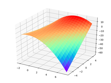
(1)较为简单的函数:
对于函数z=-(x-1)^2+5y,x区间为[-2,8].y区间为[-5,5],函数的整体二维函数图像如下所示:
使用爬山算法和遗传算法可见各自的结果为:
(1)爬山算法:最优解:25,此时各自的取值为 x=1,y= 5,全局最优
(2)遗传算法:最优解:25,此时各自的取值为 x=1,y= 5,全局最优
两者各自的最优解是一样的,均可使用
(2)较为复杂的函数:
对于函数z=-(x-1)^2+xy-2x,x区间为[-2,8].y区间为[-5,5],函数的整体二维函数图像如下所示:
函数的图像展示(可见最大值在10左右)
使用爬山算法和遗传算法可见各自的结果为:
(1)爬山算法:最优解:1.25,此时各自的取值为 x=-1.5,y= -5,为局部最优
(2)遗传算法:最优解:11.24,此时各自的取值为 x=3.5,y=5,接近全局最优
两者各自的最优解是不同的,遗传算法更加准确
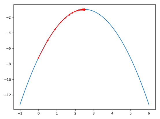
4. 附一元函数的爬山法(梯度上升法)代码:
#1-1导入相应的模块
import numpy as np
import matplotlib.pyplot as plt
#1-2定义函数的相应变量取值范围为以及函数的表达式
plot_x=np.linspace(-1,6,141)
plot_y=-(plot_x-2.5)**2-1
plt.figure()
theta=0.0
eta=0.1
erro=1e-100
theta_history=[theta]
theta1=[]
def DJ(theta):
return -2*(theta-2.5)
def J(theta):
return -(theta-2.5)**2-1
###1-3将梯度下降法封装起来成为一个梯度下降函数,以便后续的使用和调节参数,使用起来比较方便
#(其中最重要的超参数是1初始点的值x0,2梯度下降的定义步长eta,3最多的循环次数,4函数值的误差范围)
def gradient_descent(eta,theta_initial,erro=1e-8, n=1e4):
theta=theta_initial
theta_history.append(theta_initial)
i=0
while i<n:
gradient = DJ(theta)
last_theta = theta
theta = theta + gradient * eta # 梯度上升
theta_history.append(theta)
if (abs(J(theta) - J(last_theta))) < erro:
break
i+=1
def plot_theta_history():
plt.plot(plot_x,plot_y)
plt.plot(np.array(theta_history),J(np.array(theta_history)),color="r",marker="+")
plt.show()
#1-4设置自己的初始超参数,直接进行结果的输出与相应的查询
eta=0.1
x0=0.0
theta_history=[]
gradient_descent(eta,x0)
plot_theta_history()
print(len(theta_history))
print(theta_history[-1])
输出图像:(以一元二次函数为例)