简单实现一下梯度下降法。
首先引入需要的库,然后画一个简单的函数图像。
import numpy as np
import matplotlib.pyplot as plt
plot_x = np.linspace(-1,6,141) #画函数曲线,x是范围-1到6内的140个离散点
plot_y = (plot_x - 2.5)**2-1
plt.plot(plot_x,plot_y)
plt.show()

是这样一个简单的二次函数。
def dJ(theta):
return 2*(theta - 2.5) #这个是对函数进行求导,也就是斜率值
def J(theta):
return (theta - 2.5)**2 - 1 #函数,也就是plot_y
theta = 0.0
eta = 0.1 #学习步长 这个参数很重要
epsilon = 1e-8 #跳出循环的条件。当预测值与真实值之差的绝对值小于这个数就可以认为基本吻合了
while True:
gradient = dJ(theta)
last_theta = theta
theta = theta - eta * gradient
if(abs(J(theta) - J(last_theta))<epsilon):
break
print(theta)
print(J(theta))
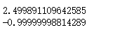
这是结果值。
如果加入一个数组存放每一个预测过的theta值,然后把过程也在图中显示出来,代码如下:
为便于调用,把函数进行封装。
def J(theta):
return (theta-2.5)**2 - 1.
def dJ(theta):
return 2*(theta-2.5)
def gradient_descent(initial_theta,eta,epsilon=1e-8):
theta = initial_theta
theta_history.append(initial_theta)
while True:
gradient = dJ(theta)
last_theta = theta
theta = theta - eta * gradient
theta_history.append(theta)
if(abs(J(theta) - J(last_theta)) < epsilon):
break
def plot_theta_history():
plt.plot(plot_x,J(plot_x))
plt.plot(np.array(theta_history),J(np.array(theta_history)),color='r',marker = '+')
plt.show()
当eta = 0.1时,图像如下:
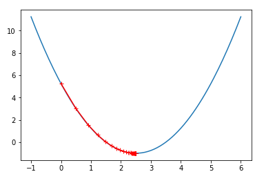
可以看出还是比较稀疏的,特别是在从0开始得到那部分,步长比较大,到后面越来越密集。
接下来改变eta的值:
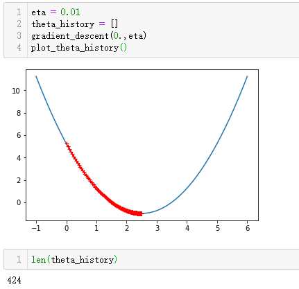
当eta=0.01时,此时数组中有424个数据,加上初始比较的那次,一共进行了425次计算步长,最终找到最小值。
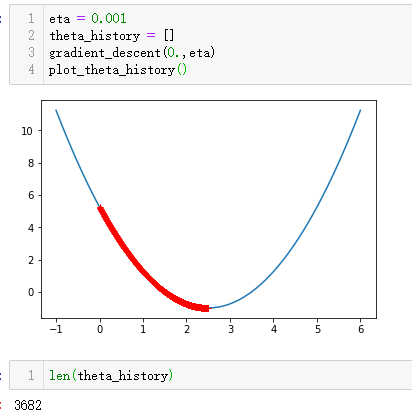

eta作为一个超参数和函数曲线上面的某一个点的斜率有关,基本上取0.01就比较合适,但是如果效果不理想,可以按照上面的方法绘图查看一下。但是不要觉得eta到1就是极限值了,这个要看实验数据和内容确定具体的eta值。