首先理解一些以下:
二分类:每一张图像输出一个类别信息
多类别分类:每一张图像输出一个类别信息
多输出分类:每一张图像输出固定个类别的信息
多标签分类:每一张图像输出类别的个数不固定,如下图所示:

多标签分类的一个重要特点就是标签是具有关联的,比如在含有sky(天空) 的图像中,极有可能含有cloud(云)、sunset(日落)等。
早期进行多标签分类使用的是Binary Cross-Entropy (BCE) or SoftMargin loss,这里我们进一步深入。
如何利用这种依赖关系来提升分类的性能?
其中之一的解决方法就是图卷积网络,例如:
Multi-Label Image Recognition with Graph Convolutional Networks
Cross-Modality Attention with Semantic Graph Embedding for Multi-Label Classification
那么什么是图呢?
图是描述对象之间关系的一种结构。对象可以用nodes(节点)表示,对象间的关系可以用edges(边)来表示,而每条边是可以带有权重的。
接下来看个例子:
假设我们现在有以下标签:sky、cloud、sunset、sea和以下样本:
1: ‘Sea’, ‘Sky’, ‘Sunset
2: ‘Sky’, ‘Sunset’
3: ‘Sky’, ‘Cloud’
4: ‘Sea’, ‘Sunset’
5: ‘Sunset’, ‘Sea’
6: ‘Sea’, ‘Sky’
7: ‘Sky’, ‘Sunset’
8: ‘Sunset’
我们可以将标签用节点表示,但是怎么表示它们之间的关系呢?我们发现有些标签总是成对出现的,可以用$P(L_{j} | L_{i})$来衡量当$L_{i}$标签出现时,$L_{j}$标签出现的可能性。
怎么将这种表示应用到我们的模型中?
使用邻接矩阵。比如:表示两标签同时出现的次数
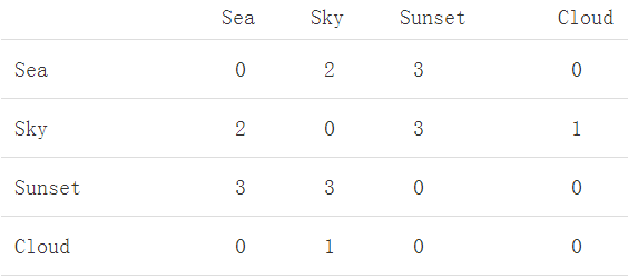
然后可以计算出每个标签出现的总次数:

接着就可以出现标签联合出现的概率了$P_{i}=A_{i}/N_{i}$,以邻接矩阵第一行为例:
p(sea,sky)=2/5=0.4 p(sea,sunset)=3/6=0.5
于是就有:
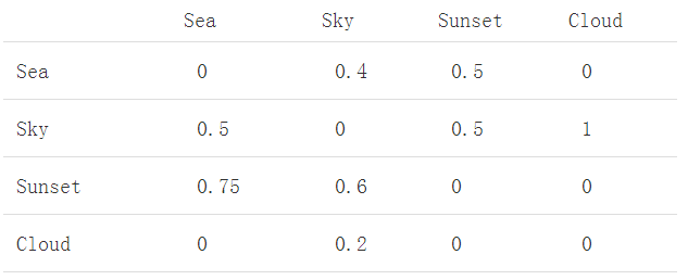
最后,别忘了将对角线置为1,因为各自发生的概率值是1.
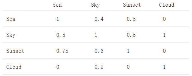
将关系用图表示:
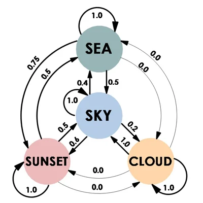
需要注意的是,
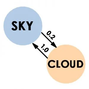
$P(L_{i} | L_{j})$ 和$P(L_{j} | L_{i})$之间的概率是不一样的。
图卷积核普通卷积的区别是什么?

图片出自:A Comprehensive Survey on Graph Neural Networks.
上图就很清楚的展示了它们之间的区别: 在卷积神经网络中,利用卷积核来提取信息。类似地,图卷积层使用特定图节点的邻居在其中定义卷积运算。 如果两个节点具有公共边缘,则它们是邻居。 在图卷积中,可学习的权重乘以特定节点(包括节点本身)的所有邻居的特征,然后在结果之上应用一些激活函数。
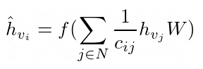
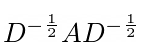
这里N是节点$v_{i}$的邻居节点的索引集(它也包括i),W是一个可学习的权重,对于邻居中的所有节点都是相同的,而f是一些非线性激活函数。$c_{ij}$是对称归一化矩阵中边缘($v_{i}$,$v_{j}$)的常数参数。 我们通过将逆度矩阵D与二进制邻接矩阵A相乘来计算此矩阵(我们将描述如何从加权后的矩阵中进一步获得二进制邻接矩阵),因此对输入图计算一次对称归一化矩阵,如下所示:
怎么定义图卷积网络?
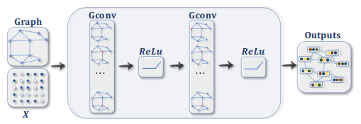
现在,我们概述在示例中将使用的整个GCN管道。 我们有一个带有С节点的图,我们想应用GCN。 图卷积运算的目标是学习输入/输出功能。 作为输入,它使用一个С×D特征矩阵(D是输入特征的维数)和一个以矩阵形式表示图形结构的加权邻接矩阵P。然后,以ReLU作为激活函数依次应用几个图卷积。 图卷积运算的输出是一个CxF特征矩阵,其中F是每个节点的输出特征数。
class GraphConvolution(nn.Module):
    """
        Simple GCN layer, similar to
        https://arxiv.org/abs/1609.02907
    """
    def __init__(self, in_features, out_features, bias=False):
        super(GraphConvolution, self).__init__()
        self.in_features = in_features
        self.out_features = out_features
        self.weight = Parameter(
                  torch.Tensor(in_features, out_features),
                  requires_grad=True)
        if bias:
            self.bias = Parameter(
                         torch.Tensor(1, 1, out_features),
                         requires_grad=True)
        else:
            self.register_parameter('bias', None)
        self.reset_parameters()

    def reset_parameters(self):
        stdv = 1. / math.sqrt(self.weight.size(1))
        self.weight.data.uniform_(-stdv, stdv)
        if self.bias is not None:
            self.bias.data.uniform_(-stdv, stdv)

    def forward(self, input, adj):
        support = torch.matmul(input.float(),
                               self.weight.float())
        output = torch.matmul(adj, support)
        if self.bias is not None:
            return output + self.bias
        else:
            return output

    def __repr__(self):
        return self.__class__.__name__ + ' (' \
               + str(self.in_features) + ' -> ' \
               + str(self.out_features) + ')'
标签向量化?
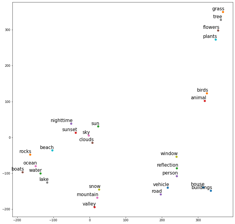
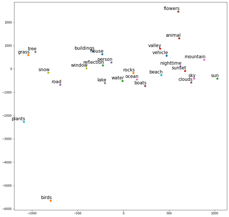
我们刚刚讨论了GCN的工作原理,以及它们如何将特征矩阵作为每个节点具有特征向量的输入。 不过,在我们的任务中,我们为标签准备任何特征,只有标签的名称。 在神经网络中处理文本时,通常使用单词的矢量表示。 每个向量在语料库(词典)的所有单词的空间中代表一个特定的单词,在该空间上已计算出该单词。 单词的空间对于找到单词之间的关系是必不可少的:向量在此空间中彼此越靠近,其含义就越接近。 看看t-SNE的功能可视化帖子,以获取有关如何从我们的数据集的小子集中为标签构建此类图像的想法。
这里可去参考:t-SNE for feature visualization post
您会看到在功能空间中具有紧密含义的单词(如天空,太阳,云彩)接近。获取此空间有多种方法:There are various approaches,在我们的示例中,我们使用基于Wikipedia的GloVe模型,特征向量的长度为300。
多标签图卷积网络:直接看原文。
We are going to implement the approach from the Multi-Label Image Recognition with Graph Convolutional Networks paper. It consists of applying all the steps described earlier:
- Calculate a weighted adjacency matrix from the training set.
- Calculate the matrix with per-label features: X=LxD
- Use vectorized labels X and weighted adjacency matrix P as the input of the graph neural network, and preprocessed image as the input for the CNN network.
- Train the model!
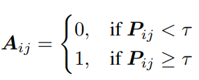
加权邻接矩阵阈值:
为了避免过度拟合,我们在加权邻接矩阵中对概率小于某个阈值τ的对(我们使用τ= 0.1)进行过滤。 我们认为这样的边缘表示不佳或错误连接。 例如,由于训练数据中的噪声,可能会发生这种情况。 例如,在我们的案例中,这种联系是“鸟”和“夜间”:它们表示随机的巧合,而不是真实的关系。
过度平滑问题:
应用图卷积层后,该节点的特征将为其自身特征与相邻节点的特征的加权总和。
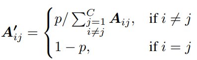
这可能会导致特定节点中的特征过度平滑,尤其是在应用了几层之后。 为了防止这种情况,我们引入了参数p,该参数用于校准分配给节点本身和其他相关节点的权重。 这样,在更新节点特征时,我们将对节点本身具有固定的权重,并且其邻居节点的权重将由邻域分布确定。 当p→1时,将不考虑节点本身的特征。 另一方面,当p→0时,邻近信息趋于被忽略。 在我们的实验中,我们使用p = 0.25。
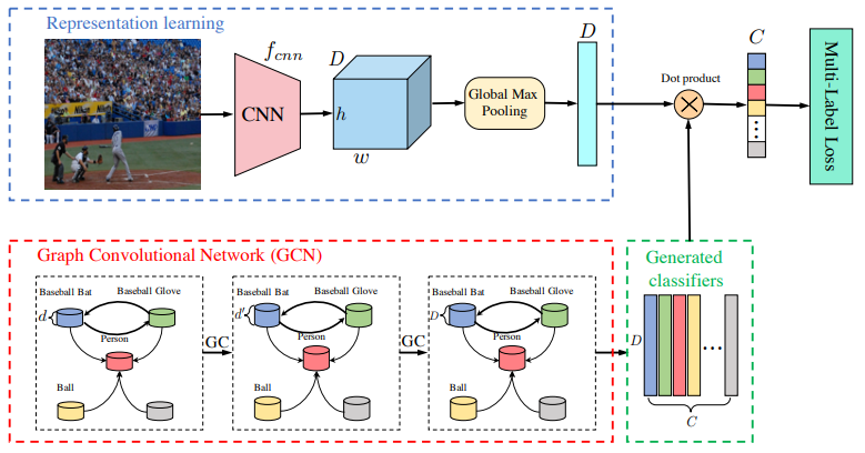
最后,让我们使用GCN构建模型。 我们将ResNeXt50的前4层用作视觉特征提取器,并将多层GCN用作标签关系提取器。 然后,通过点积运算将图像本身的特征和标签进行合并。 请参阅以下方案:
# Create adjacency matrix from statistics.
def gen_A(num_classes, t, p, adj_data):
    adj = np.array(adj_data['adj']).astype(np.float32)
    nums = np.array(adj_data['nums']).astype(np.float32)
    nums = nums[:, np.newaxis]
    adj = adj / nums
    adj[adj < t] = 0
    adj[adj >= t] = 1
    adj = adj * p / (adj.sum(0, keepdims=True) + 1e-6)
    adj = adj + np.identity(num_classes, np.int)
    return adj

# Apply adjacency matrix re-normalization trick.
def gen_adj(A):
    D = torch.pow(A.sum(1).float(), -0.5)
    D = torch.diag(D).type_as(A)
    adj = torch.matmul(torch.matmul(A, D).t(), D)
    return adj


class GCNResnext50(nn.Module):
    def __init__(self, n_classes, adj_path, in_channel=300,
                 t=0.1, p=0.25):
        super().__init__()
        self.sigm = nn.Sigmoid()

        self.features = models.resnext50_32x4d(pretrained=True)
        self.features.fc = nn.Identity()
        self.num_classes = n_classes

        self.gc1 = GraphConvolution(in_channel, 1024)
        self.gc2 = GraphConvolution(1024, 2048)
        self.relu = nn.LeakyReLU(0.2)
        # Load statistics data for adjacency matrix
        with open(adj_path) as fp:
            adj_data = json.load(fp)
        # Compute adjacency matrix
        adj = gen_A(n_classes, t, p, adj_data)
        self.A = Parameter(torch.from_numpy(adj).float(),
                           requires_grad=False)

    def forward(self, imgs, inp):
        # Get visual features from image
        feature = self.features(imgs)
        feature = feature.view(feature.size(0), -1)

        # Get graph features from graph
        inp = inp[0].squeeze()
        adj = gen_adj(self.A).detach()
        x = self.gc1(inp, adj)
        x = self.relu(x)
        x = self.gc2(x, adj)

        # We multiply the features from GCN and CNN in order to
        # take into account the contribution to the prediction of
        # classes from both the image and the graph.
        x = x.transpose(0, 1)
        x = torch.matmul(feature, x)
        return self.sigm(x)
完整代码:https://github.com/spmallick/learnopencv/tree/master/Graph-Convolutional-Networks-Model-Relations-In-Data
开始动手:
1、安装相应的包
# Install requirements
!pip install numpy scikit-image scipy scikit-learn matplotlib tqdm tensorflow torch torchvision
2、导入相关的包
import itertools
import json
import math
import os
import random
import tarfile
import time
import urllib.request
import zipfile
from shutil import copyfile

import numpy as np
import requests
import torch
from PIL import Image
from matplotlib import pyplot as plt
from numpy import printoptions
from sklearn.manifold import TSNE
from sklearn.metrics import precision_score, recall_score, f1_score
from torch import nn
from torch.nn import Parameter
from torch.utils.data.dataloader import DataLoader
from torch.utils.data.dataset import Dataset
from torch.utils.tensorboard import SummaryWriter
from torchvision import models
from torchvision import transforms
from tqdm import tqdm
3、设置随机种子
# Fix all seeds to make experiments reproducible.
torch.manual_seed(2020)
torch.cuda.manual_seed(2020)
np.random.seed(2020)
random.seed(2020)
torch.backends.cudnn.deterministic = True
4、获取数据集
# We use the .tar.gz archive from this(https://github.com/thuml/HashNet/tree/master/pytorch#datasets)
# github repository to speed up image loading(instead of loading it from Flickr).
# Let's download and extract it.
img_folder = 'images'
if not os.path.exists(img_folder):
    def download_file_from_google_drive(id, destination):
        def get_confirm_token(response):
            for key, value in response.cookies.items():
                if key.startswith('download_warning'):
                    return value
            return None

        def save_response_content(response, destination):
            CHUNK_SIZE = 32768
            with open(destination, "wb") as f:
                for chunk in tqdm(response.iter_content(CHUNK_SIZE), desc='Image downloading'):
                    if chunk:  # filter out keep-alive new chunks
                        f.write(chunk)

        URL = "https://docs.google.com/uc?export=download"
        session = requests.Session()
        response = session.get(URL, params={'id': id}, stream=True)
        token = get_confirm_token(response)

        if token:
            params = {'id': id, 'confirm': token}
            response = session.get(URL, params=params, stream=True)
        save_response_content(response, destination)

    file_id = '0B7IzDz-4yH_HMFdiSE44R1lselE'
    path_to_tar_file = str(time.time()) + '.tar.gz'
    download_file_from_google_drive(file_id, path_to_tar_file)
    print('Extraction')
    with tarfile.open(path_to_tar_file) as tar_ref:
        tar_ref.extractall(os.path.dirname(img_folder))
    os.remove(path_to_tar_file)
# Also, copy our pre-processed annotations to the dataset folder.
copyfile('/content/small_test.json', os.path.join(img_folder, 'small_test.json'))
copyfile('/content/small_train.json', os.path.join(img_folder, 'small_train.json'))
5、将标签名字用向量表示
# We want to represent our label names as vectors in order to use them as features further.
# To do that we decided to use GloVe model (https://nlp.stanford.edu/projects/glove/).
# Let's download GloVe model trained on a Wikipedia Text Corpus.
glove_zip_name = 'glove.6B.zip'
glove_url = 'http://nlp.stanford.edu/data/glove.6B.zip'
# For our purposes, we use a model where each word is encoded by a vector of length 300
target_model_name = 'glove.6B.300d.txt'
if not os.path.exists(target_model_name):
    with urllib.request.urlopen(glove_url) as dl_file:
        with open(glove_zip_name, 'wb') as out_file:
            out_file.write(dl_file.read())
    # Extract zip archive.
    with zipfile.ZipFile(glove_zip_name) as zip_f:
        zip_f.extract(target_model_name)
    os.remove(glove_zip_name)
6、加载glove模型
# Now load GloVe model.
embeddings_dict = {}

with open("glove.6B.300d.txt", 'r', encoding="utf-8") as f:
    for line in f:
        values = line.split()
        word = values[0]
        vector = np.asarray(values[1:], "float32")
        embeddings_dict[word] = vector
6、计算目标标签子集中每个标签的GloVe嵌入。
# Calculate GloVe embeddings for each label in our target label subset.
small_labels = ['house', 'birds', 'sun', 'valley',
               'nighttime', 'boats', 'mountain', 'tree', 'snow', 'beach', 'vehicle', 'rocks',
               'reflection', 'sunset', 'road', 'flowers', 'ocean', 'lake', 'window', 'plants',
               'buildings', 'grass', 'water', 'animal', 'person', 'clouds', 'sky']
vectorized_labels = [embeddings_dict[label].tolist() for label in small_labels]

# Save them for further use.
word_2_vec_path = 'word_2_vec_glow_classes.json'
with open(word_2_vec_path, 'w') as fp:
    json.dump({
        'vect_labels': vectorized_labels,
    }, fp, indent=3)
7、展示结果
%matplotlib inline
# Let's check how well GloVe represents label names from our dataset.
# It would be hard to visualize vectors with 300 values, but luckly we have t-SNE for that.
# This function builds a t-SNE model(https://www.learnopencv.com/t-sne-for-feature-visualization/)
# for label embeddings and visualizes them.
def tsne_plot(tokens, labels):
    tsne_model = TSNE(perplexity=2, n_components=2, init='pca', n_iter=25000, random_state=2020, n_jobs=4)
    new_values = tsne_model.fit_transform(tokens)
    x = []
    y = []
    for value in new_values:
        x.append(value[0])
        y.append(value[1])

    plt.figure(figsize=(13, 13))
    for i in range(len(x)):
        plt.scatter(x[i], y[i])
        plt.annotate(labels[i],
                     xy=(x[i], y[i]),
                     xytext=(5, 2),
                     size=15,
                     textcoords='offset points',
                     ha='right',
                     va='bottom')
    plt.show()
# Now we can draw t-SNE visualization.
tsne_plot(vectorized_labels, small_labels)
8、定义加载数据的类
# The Dataset class for NUS-WIDE is the same as in our previous post. The only difference
# is that we need to load vectorized representations of labels too.
class NusDatasetGCN(Dataset):
    def __init__(self, data_path, anno_path, transforms, w2v_path):
        self.transforms = transforms
        with open(anno_path) as fp:
            json_data = json.load(fp)
        samples = json_data['samples']
        self.classes = json_data['labels']

        self.imgs = []
        self.annos = []
        self.data_path = data_path
        print('loading', anno_path)
        for sample in samples:
            self.imgs.append(sample['image_name'])
            self.annos.append(sample['image_labels'])
        for item_id in range(len(self.annos)):
            item = self.annos[item_id]
            vector = [cls in item for cls in self.classes]
            self.annos[item_id] = np.array(vector, dtype=float)
        # Load vectorized labels for GCN from json.
        with open(w2v_path) as fp:
            self.gcn_inp = np.array(json.load(fp)['vect_labels'], dtype=float)

    def __getitem__(self, item):
        anno = self.annos[item]
        img_path = os.path.join(self.data_path, self.imgs[item])
        img = Image.open(img_path)
        if self.transforms is not None:
            img = self.transforms(img)
        return img, anno, self.gcn_inp

    def __len__(self):
        return len(self.imgs)
9、加载数据并显示
# Let's take a look at the data we have. To do it we need to load the dataset without augmentations.
dataset_val = NusDatasetGCN(img_folder, os.path.join(img_folder, 'small_test.json'), None, word_2_vec_path)
dataset_train = NusDatasetGCN(img_folder, os.path.join(img_folder, 'small_train.json'), None, word_2_vec_path)

# A simple function for visualization.
def show_sample(img, binary_img_labels, _):
    # Convert the binary labels back to the text representation.
    img_labels = np.array(dataset_val.classes)[np.argwhere(binary_img_labels > 0)[:, 0]]
    plt.imshow(img)
    plt.title("{}".format(', '.join(img_labels)))
    plt.axis('off')
    plt.show()

for sample_id in [13, 15, 22, 29, 57, 127]:
    show_sample(*dataset_val[sample_id])
部分结果:


10、计算标签分布
# Calculate label distribution for the entire dataset (train + test).
samples = dataset_val.annos + dataset_train.annos
samples = np.array(samples)
with printoptions(precision=3, suppress=True):
    class_counts = np.sum(samples, axis=0)
    # Sort labels according to their frequency in the dataset.
    sorted_ids = np.array([i[0] for i in sorted(enumerate(class_counts), key=lambda x: x[1])], dtype=int)
    print('Label distribution (count, class name):', list(zip(class_counts[sorted_ids].astype(int), np.array(dataset_val.classes)[sorted_ids])))
    plt.barh(range(len(dataset_val.classes)), width=class_counts[sorted_ids])
    plt.yticks(range(len(dataset_val.classes)), np.array(dataset_val.classes)[sorted_ids])
    plt.gca().margins(y=0)
    plt.grid()
    plt.title('Label distribution')
    plt.show()

11、计算邻接矩阵
# To proceed with the training we first need to compute adjacency matrix.
adj_matrix_path = 'adjacency_matrix.json'
# Count all labels.
nums = np.sum(np.array(dataset_train.annos), axis=0)
label_len = len(small_labels)
adj = np.zeros((label_len, label_len), dtype=int)
# Now iterate over the whole training set and consider all pairs of labels in sample annotation.
for sample in dataset_train.annos:
    sample_idx = np.argwhere(sample > 0)[:, 0]
    # We count all possible pairs that can be created from each sample's set of labels.
    for i, j in itertools.combinations(sample_idx, 2):
        adj[i, j] += 1
        adj[j, i] += 1

# Save it for further use.
with open(adj_matrix_path, 'w') as fp:
    json.dump({
        'nums': nums.tolist(),
        'adj': adj.tolist()
    }, fp, indent=3)
12、定义图卷积网络
# We use implementation of GCN from github repository:
# https://github.com/Megvii-Nanjing/ML-GCN/blob/master/models.py#L7
class GraphConvolution(nn.Module):
    """
        Simple GCN layer, similar to https://arxiv.org/abs/1609.02907
    """
    def __init__(self, in_features, out_features, bias=False):
        super(GraphConvolution, self).__init__()
        self.in_features = in_features
        self.out_features = out_features
        self.weight = Parameter(torch.Tensor(in_features, out_features), requires_grad=True)
        if bias:
            self.bias = Parameter(torch.Tensor(1, 1, out_features), requires_grad=True)
        else:
            self.register_parameter('bias', None)
        self.reset_parameters()

    def reset_parameters(self):
        stdv = 1. / math.sqrt(self.weight.size(1))
        self.weight.data.uniform_(-stdv, stdv)
        if self.bias is not None:
            self.bias.data.uniform_(-stdv, stdv)

    def forward(self, input, adj):
        support = torch.matmul(input.float(), self.weight.float())
        output = torch.matmul(adj, support)
        if self.bias is not None:
            return output + self.bias
        else:
            return output

    def __repr__(self):
        return self.__class__.__name__ + ' (' \
               + str(self.in_features) + ' -> ' \
               + str(self.out_features) + ')'

# Create adjacency matrix from statistics.
def gen_A(num_classes, t, p, adj_data):
    adj = np.array(adj_data['adj']).astype(np.float32)
    nums = np.array(adj_data['nums']).astype(np.float32)
    nums = nums[:, np.newaxis]
    adj = adj / nums
    adj[adj < t] = 0
    adj[adj >= t] = 1
    adj = adj * p / (adj.sum(0, keepdims=True) + 1e-6)
    adj = adj + np.identity(num_classes, np.int)
    return adj

# Apply adjacency matrix re-normalization.
def gen_adj(A):
    D = torch.pow(A.sum(1).float(), -0.5)
    D = torch.diag(D).type_as(A)
    adj = torch.matmul(torch.matmul(A, D).t(), D)
    return adj


class GCNResnext50(nn.Module):
    def __init__(self, n_classes, adj_path, in_channel=300, t=0.1, p=0.25):
        super().__init__()
        self.sigm = nn.Sigmoid()

        self.features = models.resnext50_32x4d(pretrained=True)
        self.features.fc = nn.Identity()
        self.num_classes = n_classes

        self.gc1 = GraphConvolution(in_channel, 1024)
        self.gc2 = GraphConvolution(1024, 2048)
        self.relu = nn.LeakyReLU(0.2)
        # Load data for adjacency matrix
        with open(adj_path) as fp:
            adj_data = json.load(fp)
        # Compute adjacency matrix
        adj = gen_A(n_classes, t, p, adj_data)
        self.A = Parameter(torch.from_numpy(adj).float(), requires_grad=False)

    def forward(self, imgs, inp):
        # Get visual features from image
        feature = self.features(imgs)
        feature = feature.view(feature.size(0), -1)

        # Get graph features from graph
        inp = inp[0].squeeze()
        adj = gen_adj(self.A).detach()
        x = self.gc1(inp, adj)
        x = self.relu(x)
        x = self.gc2(x, adj)

        # We multiply the features from GСN and СNN in order to take into account
        # the contribution to the prediction of classes from both the image and the graph.
        x = x.transpose(0, 1)
        x = torch.matmul(feature, x)
        return self.sigm(x)
12、定义评价指标
# Use threshold to define predicted labels and invoke sklearn's metrics with different averaging strategies.
def calculate_metrics(pred, target, threshold=0.5):
    pred = np.array(pred > threshold, dtype=float)
    return {'micro/precision': precision_score(y_true=target, y_pred=pred, average='micro'),
            'micro/recall': recall_score(y_true=target, y_pred=pred, average='micro'),
            'micro/f1': f1_score(y_true=target, y_pred=pred, average='micro'),
            'macro/precision': precision_score(y_true=target, y_pred=pred, average='macro'),
            'macro/recall': recall_score(y_true=target, y_pred=pred, average='macro'),
            'macro/f1': f1_score(y_true=target, y_pred=pred, average='macro'),
            'samples/precision': precision_score(y_true=target, y_pred=pred, average='samples'),
            'samples/recall': recall_score(y_true=target, y_pred=pred, average='samples'),
            'samples/f1': f1_score(y_true=target, y_pred=pred, average='samples'),
            }
13、初始化参数以及可视化设定
# Initialize the training parameters.
num_workers = 8 # Number of CPU processes for data preprocessing
lr = 5e-6 # Learning rate
batch_size = 32
save_freq = 1 # Save checkpoint frequency (epochs)
test_freq = 200 # Test model frequency (iterations)
max_epoch_number = 35 # Number of epochs for training
# Note: on the small subset of data overfitting happens after 30-35 epochs.

mean = [0.485, 0.456, 0.406]
std = [0.229, 0.224, 0.225]

device = torch.device('cuda')
# Save path for checkpoints.
save_path = 'chekpoints/'
# Save path for logs.
logdir = 'logs/'

# Run tensorboard.
%load_ext tensorboard
%tensorboard --logdir {logdir}
14、设置检查点
# Here is an auxiliary function for checkpoint saving.
def checkpoint_save(model, save_path, epoch):
    f = os.path.join(save_path, 'checkpoint-{:06d}.pth'.format(epoch))
    if 'module' in dir(model):
        torch.save(model.module.state_dict(), f)
    else:
        torch.save(model.state_dict(), f)
    print('saved checkpoint:', f)
15、数据预处理
# Test preprocessing.
val_transform = transforms.Compose([
    transforms.Resize((256, 256)),
    transforms.ToTensor(),
    transforms.Normalize(mean, std)
])

# Train preprocessing.
train_transform = transforms.Compose([
    transforms.Resize((256, 256)),
    transforms.RandomHorizontalFlip(),
    transforms.ColorJitter(),
    transforms.RandomAffine(degrees=20, translate=(0.2, 0.2), scale=(0.5, 1.5),
                            shear=None, resample=False,
                            fillcolor=tuple(np.array(np.array(mean) * 255).astype(int).tolist())),
    transforms.ToTensor(),
    transforms.Normalize(mean, std)
])
16、定义训练相关参数
# Initialize the dataloaders for training.
test_annotations = os.path.join(img_folder, 'small_test.json')
train_annotations = os.path.join(img_folder, 'small_train.json')

test_dataset = NusDatasetGCN(img_folder, test_annotations, val_transform, word_2_vec_path)
train_dataset = NusDatasetGCN(img_folder, train_annotations, train_transform, word_2_vec_path)

train_dataloader = DataLoader(train_dataset, batch_size=batch_size, num_workers=num_workers, shuffle=True,
                              drop_last=True)
test_dataloader = DataLoader(test_dataset, batch_size=batch_size, num_workers=num_workers)

num_train_batches = int(np.ceil(len(train_dataset) / batch_size))

# Initialize the model.
model = GCNResnext50(len(train_dataset.classes), adj_matrix_path)
# Switch model to the training mode and move it to GPU.
model.train()
model = model.to(device)

optimizer = torch.optim.Adam(model.parameters(), lr=lr)

# If more than one GPU is available we can use both to speed up the training.
if torch.cuda.device_count() > 1:
    model = nn.DataParallel(model)

os.makedirs(save_path, exist_ok=True)

# Loss function.
criterion = nn.BCELoss()
# Tensoboard logger.
logger = SummaryWriter(logdir)
17、开始训练
# Run training.
epoch = 0
iteration = 0
while True:
    batch_losses = []
    for batch_number, (imgs, targets, gcn_input) in enumerate(train_dataloader):
        imgs, targets, gcn_input = imgs.to(device), targets.to(device), gcn_input.to(device)
        optimizer.zero_grad()

        model_result = model(imgs, gcn_input)
        loss = criterion(model_result, targets.type(torch.float))

        batch_loss_value = loss.item()
        loss.backward()
        torch.nn.utils.clip_grad_norm(model.parameters(), 10.0)

        optimizer.step()

        logger.add_scalar('train_loss', batch_loss_value, iteration)
        batch_losses.append(batch_loss_value)
        with torch.no_grad():
            result = calculate_metrics(model_result.cpu().numpy(), targets.cpu().numpy())
            for metric in result:
                logger.add_scalar('train/' + metric, result[metric], iteration)

        if iteration % test_freq == 0:
            model.eval()
            with torch.no_grad():
                model_result = []
                targets = []
                for imgs, batch_targets, gcn_input in test_dataloader:
                    gcn_input = gcn_input.to(device)
                    imgs = imgs.to(device)
                    model_batch_result = model(imgs, gcn_input)
                    model_result.extend(model_batch_result.cpu().numpy())
                    targets.extend(batch_targets.cpu().numpy())

            result = calculate_metrics(np.array(model_result), np.array(targets))
            for metric in result:
                logger.add_scalar('test/' + metric, result[metric], iteration)
            print("epoch:{:2d} iter:{:3d} test: "
                  "micro f1: {:.3f} "
                  "macro f1: {:.3f} "
                  "samples f1: {:.3f}".format(epoch, iteration,
                                              result['micro/f1'],
                                              result['macro/f1'],
                                              result['samples/f1']))

            model.train()
        iteration += 1

    loss_value = np.mean(batch_losses)
    print("epoch:{:2d} iter:{:3d} train: loss:{:.3f}".format(epoch, iteration, loss_value))
    if epoch % save_freq == 0:
        checkpoint_save(model, save_path, epoch)
    epoch += 1
    if max_epoch_number < epoch:
        break
结果:
/usr/local/lib/python3.6/dist-packages/ipykernel_launcher.py:15: UserWarning: torch.nn.utils.clip_grad_norm is now deprecated in favor of torch.nn.utils.clip_grad_norm_.
  from ipykernel import kernelapp as app
/usr/local/lib/python3.6/dist-packages/sklearn/metrics/_classification.py:1272: UndefinedMetricWarning: Recall is ill-defined and being set to 0.0 in labels with no true samples. Use `zero_division` parameter to control this behavior.
  _warn_prf(average, modifier, msg_start, len(result))
/usr/local/lib/python3.6/dist-packages/sklearn/metrics/_classification.py:1272: UndefinedMetricWarning: Precision is ill-defined and being set to 0.0 in samples with no predicted labels. Use `zero_division` parameter to control this behavior.
  _warn_prf(average, modifier, msg_start, len(result))
epoch: 0 iter:  0 test: micro f1: 0.131 macro f1: 0.124 samples f1: 0.121
/usr/local/lib/python3.6/dist-packages/sklearn/metrics/_classification.py:1272: UndefinedMetricWarning: Precision is ill-defined and being set to 0.0 in labels with no predicted samples. Use `zero_division` parameter to control this behavior.
  _warn_prf(average, modifier, msg_start, len(result))
/usr/local/lib/python3.6/dist-packages/sklearn/metrics/_classification.py:1515: UndefinedMetricWarning: F-score is ill-defined and being set to 0.0 in labels with no true nor predicted samples. Use `zero_division` parameter to control this behavior.
  average, "true nor predicted", 'F-score is', len(true_sum)
/usr/local/lib/python3.6/dist-packages/sklearn/metrics/_classification.py:1272: UndefinedMetricWarning: Precision is ill-defined and being set to 0.0 due to no predicted samples. Use `zero_division` parameter to control this behavior.
  _warn_prf(average, modifier, msg_start, len(result))
epoch: 0 iter:156 train: loss:0.273
saved checkpoint: chekpoints/checkpoint-000000.pth
epoch: 1 iter:200 test: micro f1: 0.478 macro f1: 0.140 samples f1: 0.421
epoch: 1 iter:312 train: loss:0.170
saved checkpoint: chekpoints/checkpoint-000001.pth
epoch: 2 iter:400 test: micro f1: 0.594 macro f1: 0.225 samples f1: 0.564
epoch: 2 iter:468 train: loss:0.150
saved checkpoint: chekpoints/checkpoint-000002.pth
epoch: 3 iter:600 test: micro f1: 0.630 macro f1: 0.272 samples f1: 0.605
epoch: 3 iter:624 train: loss:0.139
saved checkpoint: chekpoints/checkpoint-000003.pth
epoch: 4 iter:780 train: loss:0.131
saved checkpoint: chekpoints/checkpoint-000004.pth
epoch: 5 iter:800 test: micro f1: 0.678 macro f1: 0.386 samples f1: 0.654
epoch: 5 iter:936 train: loss:0.125
saved checkpoint: chekpoints/checkpoint-000005.pth
epoch: 6 iter:1000 test: micro f1: 0.679 macro f1: 0.413 samples f1: 0.650
epoch: 6 iter:1092 train: loss:0.120
saved checkpoint: chekpoints/checkpoint-000006.pth
epoch: 7 iter:1200 test: micro f1: 0.688 macro f1: 0.446 samples f1: 0.655
epoch: 7 iter:1248 train: loss:0.116
saved checkpoint: chekpoints/checkpoint-000007.pth
epoch: 8 iter:1400 test: micro f1: 0.703 macro f1: 0.491 samples f1: 0.678
epoch: 8 iter:1404 train: loss:0.112
saved checkpoint: chekpoints/checkpoint-000008.pth
epoch: 9 iter:1560 train: loss:0.109
saved checkpoint: chekpoints/checkpoint-000009.pth
epoch:10 iter:1600 test: micro f1: 0.697 macro f1: 0.485 samples f1: 0.669
epoch:10 iter:1716 train: loss:0.107
saved checkpoint: chekpoints/checkpoint-000010.pth
epoch:11 iter:1800 test: micro f1: 0.714 macro f1: 0.546 samples f1: 0.693
epoch:11 iter:1872 train: loss:0.103
saved checkpoint: chekpoints/checkpoint-000011.pth
epoch:12 iter:2000 test: micro f1: 0.705 macro f1: 0.526 samples f1: 0.678
epoch:12 iter:2028 train: loss:0.101
saved checkpoint: chekpoints/checkpoint-000012.pth
epoch:13 iter:2184 train: loss:0.098
saved checkpoint: chekpoints/checkpoint-000013.pth
epoch:14 iter:2200 test: micro f1: 0.700 macro f1: 0.523 samples f1: 0.674
epoch:14 iter:2340 train: loss:0.096
saved checkpoint: chekpoints/checkpoint-000014.pth
epoch:15 iter:2400 test: micro f1: 0.711 macro f1: 0.541 samples f1: 0.689
epoch:15 iter:2496 train: loss:0.093
saved checkpoint: chekpoints/checkpoint-000015.pth
epoch:16 iter:2600 test: micro f1: 0.706 macro f1: 0.532 samples f1: 0.681
epoch:16 iter:2652 train: loss:0.091
saved checkpoint: chekpoints/checkpoint-000016.pth
epoch:17 iter:2800 test: micro f1: 0.715 macro f1: 0.559 samples f1: 0.692
epoch:17 iter:2808 train: loss:0.089
saved checkpoint: chekpoints/checkpoint-000017.pth
epoch:18 iter:2964 train: loss:0.086
saved checkpoint: chekpoints/checkpoint-000018.pth
epoch:19 iter:3000 test: micro f1: 0.710 macro f1: 0.545 samples f1: 0.686
epoch:19 iter:3120 train: loss:0.084
saved checkpoint: chekpoints/checkpoint-000019.pth
epoch:20 iter:3200 test: micro f1: 0.712 macro f1: 0.553 samples f1: 0.682
epoch:20 iter:3276 train: loss:0.082
saved checkpoint: chekpoints/checkpoint-000020.pth
epoch:21 iter:3400 test: micro f1: 0.711 macro f1: 0.553 samples f1: 0.686
epoch:21 iter:3432 train: loss:0.080
saved checkpoint: chekpoints/checkpoint-000021.pth
epoch:22 iter:3588 train: loss:0.078
saved checkpoint: chekpoints/checkpoint-000022.pth
epoch:23 iter:3600 test: micro f1: 0.712 macro f1: 0.556 samples f1: 0.689
epoch:23 iter:3744 train: loss:0.077
saved checkpoint: chekpoints/checkpoint-000023.pth
epoch:24 iter:3800 test: micro f1: 0.708 macro f1: 0.553 samples f1: 0.682
epoch:24 iter:3900 train: loss:0.074
saved checkpoint: chekpoints/checkpoint-000024.pth
epoch:25 iter:4000 test: micro f1: 0.714 macro f1: 0.561 samples f1: 0.691
epoch:25 iter:4056 train: loss:0.072
saved checkpoint: chekpoints/checkpoint-000025.pth
epoch:26 iter:4200 test: micro f1: 0.713 macro f1: 0.564 samples f1: 0.689
epoch:26 iter:4212 train: loss:0.070
saved checkpoint: chekpoints/checkpoint-000026.pth
epoch:27 iter:4368 train: loss:0.069
saved checkpoint: chekpoints/checkpoint-000027.pth
epoch:28 iter:4400 test: micro f1: 0.709 macro f1: 0.555 samples f1: 0.687
epoch:28 iter:4524 train: loss:0.066
saved checkpoint: chekpoints/checkpoint-000028.pth
epoch:29 iter:4600 test: micro f1: 0.711 macro f1: 0.559 samples f1: 0.689
epoch:29 iter:4680 train: loss:0.064
saved checkpoint: chekpoints/checkpoint-000029.pth
epoch:30 iter:4800 test: micro f1: 0.714 macro f1: 0.579 samples f1: 0.698
epoch:30 iter:4836 train: loss:0.063
saved checkpoint: chekpoints/checkpoint-000030.pth
epoch:31 iter:4992 train: loss:0.061
saved checkpoint: chekpoints/checkpoint-000031.pth
epoch:32 iter:5000 test: micro f1: 0.707 macro f1: 0.564 samples f1: 0.681
epoch:32 iter:5148 train: loss:0.059
saved checkpoint: chekpoints/checkpoint-000032.pth
epoch:33 iter:5200 test: micro f1: 0.699 macro f1: 0.556 samples f1: 0.679
epoch:33 iter:5304 train: loss:0.058
saved checkpoint: chekpoints/checkpoint-000033.pth
epoch:34 iter:5400 test: micro f1: 0.706 macro f1: 0.565 samples f1: 0.685
epoch:34 iter:5460 train: loss:0.055
saved checkpoint: chekpoints/checkpoint-000034.pth
epoch:35 iter:5600 test: micro f1: 0.706 macro f1: 0.564 samples f1: 0.686
epoch:35 iter:5616 train: loss:0.055
saved checkpoint: chekpoints/checkpoint-000035.pth
最后是进行测试:
# Run inference on the test data.
model.eval()
for sample_id in [1, 2, 3, 4, 6]:
    test_img, test_labels, gcn_input  = test_dataset[sample_id]
    test_img_path = os.path.join(img_folder, test_dataset.imgs[sample_id])
    with torch.no_grad():
        raw_pred = model(test_img.unsqueeze(0).cuda(), torch.from_numpy(gcn_input).unsqueeze(0).cuda()).cpu().numpy()[0]
        raw_pred = np.array(raw_pred > 0.5, dtype=float)

    predicted_labels = np.array(dataset_val.classes)[np.argwhere(raw_pred > 0)[:, 0]]
    if not len(predicted_labels):
        predicted_labels = ['no predictions']
    img_labels = np.array(dataset_val.classes)[np.argwhere(test_labels > 0)[:, 0]]
    plt.imshow(Image.open(test_img_path))
    plt.title("Predicted labels: {} \nGT labels: {}".format(', '.join(predicted_labels), ', '.join(img_labels)))
    plt.axis('off')
    plt.show()


参考:https://www.learnopencv.com/graph-convolutional-networks-model-relations-in-data/