tensorflow学习笔记第一部分

学习地址：Tensorflow 搭建自己的神经网络 (莫烦 Python 教程)_哔哩哔哩 (゜-゜)つロ 干杯~-bilibili  https://www.bilibili.com/video/av16001891/?p=16

第一课：

#-*- coding: utf-8 -*-
import tensorflow as tf
import numpy as np

#creat data
x_data=np.random.rand(100).astype(np.float32)
y_data=x_data*0.1+0.3
'''
随机生成x和y 数据，x_data的数据类型为32位浮点数，x为100个数据
'''

#create tesorflow structure start#
Weights=tf.Variable(tf.random_uniform([1],-1.0,1.0))
biases=tf.Variable(tf.zeros([1]))

y=Weights*x_data+biases

loss=tf.reduce_mean(tf.square(y-y_data))
optimizer=tf.train.GradientDescentOptimizer(0.5)
train=optimizer.minimize(loss)

init=tf.initialize_all_variables()
#create tensorflow structure end#
'''
weights所表示的是随机变量，里面参数是随机数列生成方式，[1]是一维的意思，生成范围是-1.0到1.0
biases初始值是零
optimizer是gradientdecentoptimizer类型的优化器,是最基础类型的优化器，里面的参数0.5是learning rate
init是初始化所有的值，建立了变量
'''
#这个session很牛逼的样子，用session来运行这个tensorflow-structure里面的某个部分比如train，访问Weights
sess=tf.Session()
sess.run(init)#very important


for step in range(201):
    sess.run(train)
    if step%20==0:
        print(step,sess.run(Weights),sess.run(biases))

'''
记住sess.run(train)这样的
要访问weights要用这样的样子来访问，sess.run(Weighs)
'''

第一课运行结果：Instructions for updating:
Use `tf.global_variables_initializer` instead.
0 [-0.05082199] [0.5134365]
20 [0.03446221] [0.33414757]
40 [0.0791579] [0.3108595]
60 [0.09337187] [0.3034535]
80 [0.09789216] [0.3010983]
100 [0.09932968] [0.30034927]
120 [0.09978682] [0.3001111]
140 [0.09993222] [0.30003533]
160 [0.09997844] [0.30001125]
180 [0.09999314] [0.3000036]

200 [0.09999783] [0.30000114]

第二课：

#-*- coding: utf-8 -*-
import tensorflow as tf
import numpy as np

matrix1=tf.constant([[3,3]])
matrix2=tf.constant([[2],
                     [2]])
product=tf.matmul(matrix1,matrix2)#matmul is short of matrix mutiply
'''
mat1是1*1矩阵，mat2是2*1矩阵
product是两个矩阵的相乘，类比到numpy中也就是np.dot(m1,m2)
'''

###method 1
##sess= tf.Session()
##result=sess.run(product)
##print(result)
#sess.close()

#method 2
with tf.Session() as sess:
    result2=sess.run(product)
    print(result2)


'''
方法1和方法2互相替代，访问tf中的东西都需要用tf.Session来访问，且访问完需要close,如果使用with as，则可以省略close,记住这个with assession
'''

第二课运行结果:>>>[[12]]

第三课：

#-*- coding: utf-8 -*-
import tensorflow as tf

state=tf.Variable(0,name='counter')
#print(state.name)
one=tf.constant(1)
'''
state是tf的变量，起始数值为0，还可以取名为counter
one是tf的常量，数值为1
print（state.name）出来的是name:value
'''

new_value=tf.add(state,one)
update=tf.assign(state,new_value)

init=tf.initialize_all_variables()#must have if defining variable
'''
new_value是state和one之和，tf里的加法是tf.add(val1,val2)
tf.assign(state,new_value)是把new_value里的变量加载到state中
等下一次运算的时候，第二个state再加上1变成new_value，说不太清，自己感受一下
assign(val1，val2)是assign val2 to val1
'''

with tf.Session() as sess:
    sess.run(init)
    for _ in range(3):
        sess.run(update)
        print(sess.run(state))

'''
只要tf中有变量，就一定要tf.initialize_all_variables
再在sess中run(inint)，不断用session运行update,并session获得state打印出来
'''

第三课运行结果：Instructions for updating:
Use `tf.global_variables_initializer` instead.
1
2

3

第四课：

#-*- coding: utf-8 -*-
import tensorflow as tf

input1=tf.placeholder(tf.float32)
input2=tf.placeholder(tf.float32)

output=tf.multiply(input1,input2)
'''
input1和2是tf的储存数据的holder,output是tf相乘input1和input2的值
'''

with tf.Session() as sess:
    print(sess.run(output,feed_dict={input1:[7.],input2:[2.]}))
'''
因为input1和2是placeholder的话，所以sess.run里面需要有feed_dict
来接收传进来的数值给input1和2，用dic的形式输入7和2给input1和2
用placeholder的时候就要在session.run的时候feed_dic
'''

第四课运行结果：>>> [14.]

第五课：

#-*- coding: utf-8 -*-
import tensorflow as tf
import numpy as np

#添加神经层来修改激活值大小

def add_layer(inputs,in_size,out_size,activation_function=None):
    Weights=tf.Variable(tf.random_normal([in_size,out_size]))
    biases=tf.Variable(tf.zeros([1,out_size])+0.1)
    Wx_plus_b=tf.matmul(inputs,Weights)+biases
    if activation_function is None:
        outputs=Wx_plus_b
    else:
        outputs=activation_function(Wx_plus_b)
    return outputs
    
'''
如果传入的激活方程为None，则这一层layer相当于没用，input=output
否则输出等于经过activation_function变化的值
Wx_plus_b是预测值，还没有被激活的值，为啥里面是random?
weights是in_size行out_size列的随机值，biases是一行out_size列的非零列向量
（biases在机器学习中推荐不为0）
'''

x_data=np.linspace(-1,1,300)[:,np.newaxis]
noise=np.random.normal(0,0.05,x_data.shape)
y_data=np.square(x_data)-0.5+noise

#x_data和y_data 是样本数据，x_data 被弄成三百行一列，y则是x平方减去0.5加上噪点

#xs和ys被后面用来train当容器用的，先不用管
xs=tf.placeholder(tf.float32,[None,1])
ys=tf.placeholder(tf.float32,[None,1])


l1=add_layer(xs,1,10,activation_function=tf.nn.relu)#调用上面弄到的增加一层layer,返回激励函数后的outputs
prediction=add_layer(l1,10,1,activation_function=None)#预测值是prediction

loss=tf.reduce_mean(tf.reduce_sum(tf.square(ys-prediction),
                                  reduction_indices=[1]))
#reduction_indices在tensorflow1.0后被改为axis，网上有改成reduc_in=1的
train_step=tf.train.GradientDescentOptimizer(0.1).minimize(loss)#使用这个其实就在更改bias和weighs

init=tf.initialize_all_variables()
sess=tf.Session()
sess.run(init)
'''
运行1000次train_step,迭代一千次
'''
for i in range(1000):
    sess.run(train_step,feed_dict={xs:x_data,ys:y_data})
    if not i%50:
        print(sess.run(loss,feed_dict={xs:x_data,ys:y_data}))

运行结果：WARNING:tensorflow:From C:\python364\lib\site-packages\tensorflow\python\util\tf_should_use.py:118: initialize_all_variables (from tensorflow.python.ops.variables) is deprecated and will be removed after 2017-03-02.
Instructions for updating:
Use `tf.global_variables_initializer` instead.
0.6017571
0.008654009
0.0066226027
0.0060757496
0.005787913
0.005604301
0.0054377895
0.00529302
0.0051547633
0.005016695
0.004909197
0.004790244
0.0046654823
0.0045420392
0.0044349297
0.004340439
0.0042645116
0.004198417
0.004132898
0.0040747593

>>> 

第五课还有点不太理解。。估计以后会理解，先继续学

第六课到第十课内容简介:

第六课:

#-*- coding: utf-8 -*-
import tensorflow as tf
import numpy as np
import matplotlib.pyplot as plt

#添加神经层来修改激活值大小
#add one more layer and return the outputs of this layer
def add_layer(inputs,in_size,out_size,activation_function=None):
    Weights=tf.Variable(tf.random_normal([in_size,out_size]))
    biases=tf.Variable(tf.zeros([1,out_size])+0.1)
    Wx_plus_b=tf.matmul(inputs,Weights)+biases
    if activation_function is None:
        outputs=Wx_plus_b
    else:
        outputs=activation_function(Wx_plus_b)
    return outputs
    
'''
如果传入的激活方程为None，则这一层layer相当于没用，input=output
否则输出等于经过activation_function变化的值
Wx_plus_b是预测值，还没有被激活的值，为啥里面是random?
weights是in_size行out_size列的随机值，biases是一行out_size列的非零列向量
（biases在机器学习中推荐不为0）
'''
#make up some real data
x_data=np.linspace(-1,1,300)[:,np.newaxis]
noise=np.random.normal(0,0.05,x_data.shape)
y_data=np.square(x_data)-0.5+noise

#x_data和y_data 是样本数据，x_data 被弄成三百行一列，y则是x平方减去0.5加上噪点

#xs和ys被后面用来train当容器用的，先不用管,define placeholder for inputs to network
xs=tf.placeholder(tf.float32,[None,1])
ys=tf.placeholder(tf.float32,[None,1])

#add hidden layer
l1=add_layer(xs,1,10,activation_function=tf.nn.relu)#调用上面弄到的增加一层layer,返回激励函数后的outputs
#add output layer
prediction=add_layer(l1,10,1,activation_function=None)#预测值是prediction
#the error between prediction and real data
loss=tf.reduce_mean(tf.reduce_sum(tf.square(ys-prediction),
                                  reduction_indices=[1]))
#reduction_indices在tensorflow1.0后被改为axis，网上有改成reduc_in=1的
train_step=tf.train.GradientDescentOptimizer(0.1).minimize(loss)#使用这个其实就在更改bias和weighs

init=tf.initialize_all_variables()
sess=tf.Session()
sess.run(init)


#显示figure,内容为x_data和y_data(make up some real data中的)
fig=plt.figure()
ax=fig.add_subplot(1,1,1)
ax.scatter(x_data,y_data)
plt.ion()#plt可以连续
plt.show()

#运行1000次train_step,迭代一千次
for i in range(1000):
    sess.run(train_step,feed_dict={xs:x_data,ys:y_data})
    if not i%50:
        #print(sess.run(loss,feed_dict={xs:x_data,ys:y_data}))
        try:
            ax.lines.remove(lines[0])#移掉之前的线，否则线会重合
        except Exception:
            pass
        prediction_value=sess.run(prediction,feed_dict={xs:x_data})
        lines=ax.plot(x_data,prediction_value,'r-',lw=5)
        plt.pause(0.1)

第七课:

#-*- coding: utf-8 -*-
import tensorflow as tf
import numpy as np

#添加神经层来修改激活值大小

def add_layer(inputs,in_size,out_size,activation_function=None):
    with tf.name_scope('layer'):
        with tf.name_scope('weights'):
            Weights=tf.Variable(tf.random_normal([in_size,out_size]),name='W')
        with tf.name_scope('biases'):
            biases=tf.Variable(tf.zeros([1,out_size])+0.1,name='b')
        with tf.name_scope('Wx_plus_b'):
            Wx_plus_b=tf.add(tf.matmul(inputs,Weights),biases)
        #先忽略activation
        if activation_function is None:
            outputs=Wx_plus_b
        else:
            outputs=activation_function(Wx_plus_b)
        return outputs
    
#详情请见figure1,x_input对应图中x_input,整个with name_scope对应中红色大框架
with tf.name_scope('inputs'):
    xs=tf.placeholder(tf.float32,[None,1],name='x_input')
    ys=tf.placeholder(tf.float32,[None,1],name='y_niput')


l1=add_layer(xs,1,10,activation_function=tf.nn.relu)#调用上面弄到的增加一层layer,返回激励函数后的outputs
prediction=add_layer(l1,10,1,activation_function=None)#预测值是prediction
with tf.name_scope('loss'):#这些后面可以加上name来描述
    loss=tf.reduce_mean(tf.reduce_sum(tf.square(ys-prediction),
                                      reduction_indices=[1]))
#reduction_indices在tensorflow1.0后被改为axis，网上有改成reduc_in=1的
with tf.name_scope('train'):
    train_step=tf.train.GradientDescentOptimizer(0.1).minimize(loss)#使用这个其实就在更改bias和weighs

sess=tf.Session()
#把整个框架加载到文件里，再打开浏览器才能观看,graph是整个框架
#修改：tf.get_default_graph()原本是sess.graph
writer=tf.summary.FileWriter("./",tf.get_default_graph())
#或者下面两行直接sess.run(tf.initialize_all_variables)
init=tf.initialize_all_variables()
sess.run(init)
print('ok')
'''
上面writer里的地址是文件产生的地址，需要用TensorBoard打开则需要先cd到文件下，
接着终端输入：tensorboard --logdir =路径，打开浏览器打开即可
打开的网站里面的graphs里就是视图了
'''

figure1:

第八课:

#-*- coding: utf-8 -*-
'''
从上一节课的延伸讲解用视图查看训练过程
这节课比上节课多出histogram的部分来查看训练过程loss的变化过程
想在视图histogram查看到的内容，都在后面加上histogram_summary语句，详情见代码
'''
import tensorflow as tf
import numpy as np


def add_layer(inputs,in_size,out_size,n_layer,activation_function=None):
    #add a layer
    layer_name='layer%s'%n_layer
    #传进来的layer_name，是这节课新加的,后面的每个layer_name都是这节课加的
    with tf.name_scope(layer_name):
        with tf.name_scope('weights'):
            Weights=tf.Variable(tf.random_normal([in_size,out_size]),name='W')
            tf.summary.histogram(layer_name+'/weights',Weights)
            #显示layer_name和weights
            #网上说tf.summary.histogram(layer_name+"/biases",biases)
            #原来代码：tf.histogram_summary
        with tf.name_scope('biases'):
            biases=tf.Variable(tf.zeros([1,out_size])+0.1,name='b')
            tf.summary.histogram(layer_name+'/biases',biases)
        with tf.name_scope('Wx_plus_b'):
            Wx_plus_b=tf.add(tf.matmul(inputs,Weights),biases)
        #先忽略activation
        if activation_function is None:
            outputs=Wx_plus_b
        else:
            outputs=activation_function(Wx_plus_b,)
        tf.summary.histogram(layer_name+'/outputs',outputs)
        return outputs
    
#make up some real data
#比上节课多出来的部分
x_data=np.linspace(-1,1,300)[:,np.newaxis]
noise=np.random.normal(0,0.05,x_data.shape)
y_data=np.square(x_data)-0.5+noise
    
with tf.name_scope('inputs'):
    xs=tf.placeholder(tf.float32,[None,1],name='x_input')
    ys=tf.placeholder(tf.float32,[None,1],name='y_niput')


l1=add_layer(xs,1,10,n_layer=1,activation_function=tf.nn.relu)
prediction=add_layer(l1,10,1,n_layer=2,activation_function=None)


with tf.name_scope('loss'):
    loss=tf.reduce_mean(tf.reduce_sum(tf.square(ys-prediction),
                                      reduction_indices=[1]))
    tf.summary.scalar('loss',loss)
    #这个是一个量的变换，不在histogram,而是在视图Event里观看loss的变化
    #网上说现在是tf.summary.scalar('loss',loss),格式是tf.summary.**()
    #源代码：tf.scalar_summary
#reduction_indices在tensorflow1.0后被改为axis，网上有改成reduc_in=1的
with tf.name_scope('train'):
    train_step=tf.train.GradientDescentOptimizer(0.1).minimize(loss)

sess=tf.Session()
merged=tf.summary.merge_all()
#merge_all_summaries新版本改成了tf.summary.merge_all
#打包好后把所有summary打包到merged，弄到writer里面
writer=tf.summary.FileWriter("./",tf.get_default_graph())
init=tf.initialize_all_variables()
sess.run(init)
'''
上面writer里的地址是文件产生的地址，需要用TensorBoard打开则需要先cd到文件下，
接着终端输入：tensorboard --logdir =路径，打开浏览器打开即可
打开的网站里面的graphs里就是视图了
'''
for i in range(1000):
    sess.run(train_step,feed_dic={xs:x_data,ys:y_data})
    if i%50==0:
        #五十步发挥一次merged作用
        result=sess.run(merged,
                        feed_dict={xs:x_data,ys:y_data})
        writer.add_summary(result,i)
        #网上说tf.summary.merge_all

'''
报错:
    sess.run(train_step,feed_dic={xs:x_data,ys:y_data})
TypeError: run() got an unexpected keyword argument 'feed_dic'
还不知道怎么改，先跳过
'''

第九课:

#-*- coding: utf-8 -*-
import tensorflow as tf
import numpy as np
from tensorflow.examples.tutorials.mnist import input_data
#number 1 to 10 data,
#加载mnist数据，
mnist=input_data.read_data_sets('MNIST_data',one_hot=True)

def compute_accuracy(v_xs,v_ys):
    '''
    把vv_xs弄到prediction里面生成预测值（一行十列概率值）
    correct_prediction里面对比真实数据和预测值每个位置是否相等
    accuracy这组数据中计算有几个对的
    result输出的是百分比
    '''
    global prediction
    y_pre=sess.run(prediction,feed_dict={xs:v_xs})
    correct_prediction=tf.equal(tf.argmax(y_pre,1),tf.argmax(v_ys,1))
    accuracy=tf.reduce_mean(tf.cast(correct_prediction,tf.float32))
    result=sess.run(accuracy,feed_dict={xs:v_xs,ys:v_ys})
    return result

def add_layer(inputs,in_size,out_size,activation_function=None,):
    #add one more layer and return the output of this layer
    Weights=tf.Variable(tf.random_normal([in_size,out_size]))
    biases=tf.Variable(tf.zeros([1,out_size])+0.1)
    Wx_plus_b=tf.matmul(inputs,Weights)+biases
    if activation_function is None:
        outputs=Wx_plus_b
    else:
        outputs=activation_function(Wx_plus_b,)
    return outputs


#define placeholder for inputs to network
xs=tf.placeholder(tf.float32,[None,784])#784是每张图片有784个像素点()28*28
ys=tf.placeholder(tf.float32,[None,10])#y有十个输出（？）


#add output layer
prediction=add_layer(xs,784,10,activation_function=tf.nn.softmax)
#softmax一般是用来做classfication的

#the error between prediction and real data(loss)
#和以前的loss不太一样，cross_enctropy组合softmax是classfication算法
cross_enctropy=tf.reduce_mean(-tf.reduce_sum(ys*tf.log(prediction),
                                             reduction_indices=[1]))

sess=tf.Session()

sess.run(tf.initialize_all_variables())
#随机梯度下降
for i in range(1000):
    batch_xs,batch_ys=mnist.train.next_batch(100)
    sess.run(train_step,feed_dict={xs:batch_xs,ys:batch_ys})
    if i%50==0:
        print(compute_accuracy(
            mnist.test.images,mnist.test.labels))

'''
错误：连接不上mnist下载
演示的例子：0.2->0.4一直->0.87
'''

第十课:

#-*- coding: utf-8 -*-
'''
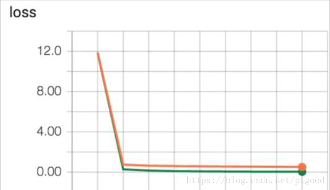
这一课好像是教解决overfitting的问题,用dropout的方法,过拟合的loss和训练次数图见figure2
实际上dropout是对add_layer中的Wx_plus_b舍弃值来,
标记有星星之前的是被运用dropout之前的程序
'''
import tensorflow as tf
from sklearn.datasets import load_digits
from sklearn.cross_validation import train_test_split
from sklearn.preprocessing import LabelBinarizer
#load data
#X=digits.data是从零到九的数字图片data,
digits=load_digits()
X=digits.data
y=LabelBinarizer().fit_transfrom(y)
#y是在表示数字的数据,类似于mnist里的数据
#把数据分为X_train和X_test
X_train,X_test,y_train,y_test=train_test_split(X,y,test_size=.3)

def add_layer(inputs,in_size,out_size,activation_function=None):
    with tf.name_scope('layer'):
        with tf.name_scope('weights'):
            Weights=tf.Variable(tf.random_normal([in_size,out_size]),name='W')
        with tf.name_scope('biases'):
            biases=tf.Variable(tf.zeros([1,out_size])+0.1,name='b')
        with tf.name_scope('Wx_plus_b'):
            Wx_plus_b=tf.add(tf.matmul(inputs,Weights),biases)
            Wx_plus_b=tf.nn.dropout(Wx_plus_b,keep_prob)#星星,这个是dropout核心
        
        if activation_function is None:
            outputs=Wx_plus_b
        else:
            outputs=activation_function(Wx_plus_b)
        tf.histogram_summary(layer_name+'/outputs',outputs)
        #这句不加up主说报错
        return outputs

#define placeholder for inputs to network
keep_prob=tf.placeholder(tf.float32)#星星
#keep probability,保持多少的值不被dropout掉
xs=tf.placeholder(tf.float32,[None,64])#8*8
ys=tf.placeholder(tf.float32,[None,10])

#add output layer
#一个隐藏层,一个输出层,skldata中data是64个单位,所以input_size=64
#activation_f的使用是up主的原因
l1=add_layer(xs,64,50,'l1',activation_function=tf.nn.tanh)#8*8
prediction=add_layer(l1,50,10,'l2',activation_function=tr.nn.softmax)
#the loss between prediction and real data
cross_entropy=tf.reduce_mean(-tf.reduce_sum(ys*tf.log(prediction),
                                            reduction_indices=[1]))
#sklearn.cross_validation已经被弃用 用sklearn.model_selection替代
#cross_entropy实际是loss,再把这个放入summary中,在在Tensorboard中显示
tf.scalar_summary('loss',cross_entropy)
train_step=tf.train.GradientDescentOptimizer(0.6).minimize(cross_entropy)

sess=tf.Session()
merged=tf.merge_all_summaries()
#summary writer goes in there
train_writer=tf.train.SummaryWriter("./train",sess.graph)
test_writer=tf.train.SummaryWriter("./test",sess.graph)
#要记录两个summary:test 和train,
#网上说tf.train.SummaryWriter已弃用，需要改成tf.summary.FileWriter

sess.run(tf.initialize_all_variables())
#initialize_all_variables已被弃用，使用tf.global_variables_initializer()代替。

for i in range(500):
    sess.run(train_step,feed_dict={xs:X_train,ys:y_train,keep_pro:0.5})#星星,改成1可以看到dropout前的
    if i%50==0:
        #record loss
        train_result=sess.run(merged,fed_dict={xs:X_train,ys:train,keep_pro:1})#星星
        test_result=sess.run(merged,fed_dict={xs:X_train,ys:train,keep_pro:1})#星星
        train_writer,add_summary(train_result,i)
        test_writer,add_summary(test_result,i)

figure2: