文章目录
文章推荐:
数据可视化——利用pandas和seaborn绘图基础
利用python进行数据分析——第十章.GroupBy机制(数据聚合与分组操作)
利用python进行数据分析——第十一章时间序列
一.分类数据
这一节介绍的是pandas的Categorical类型。我会向你展示通过使用它,提高性能和内存的使用率。我还会介绍一些在统计和机器学习中使用分类数据的工具。
1.1 背景和目标
表中的一列通常会有重复的包含不同值的小集合的情况。我们已经学过了unique和value_counts,它们可以从数组提取出不同的值,并分别计算频率:
import numpy as np
import pandas as pd
values = pd.Series(['apple','orange','apple','apple'] * 2)
values
0     apple
1    orange
2     apple
3     apple
4     apple
5    orange
6     apple
7     apple
dtype: object
pd.unique(values)
array(['apple', 'orange'], dtype=object)
pd.value_counts(values)
apple     6
orange    2
dtype: int64
许多数据系统(数据仓库、统计计算或其它应用)都发展出了特定的表征重复值的方法,以进行高效的存储和计算。在数据仓库中,最好的方法是使用所谓的包含不同值的维表(Dimension Table),将主要的参数存储为引用维表整数键:
values = pd.Series([0, 1, 0, 0 ] * 2)
dim = pd.Series(['apple','orange'])
values
0    0
1    1
2    0
3    0
4    0
5    1
6    0
7    0
dtype: int64
dim
0     apple
1    orange
dtype: object
可以使用take方法存储原始的字符串Series
dim.take(values)
0     apple
1    orange
0     apple
0     apple
0     apple
1    orange
0     apple
0     apple
dtype: object
这种用整数表示的方法称为分类或字典编码表示法。不同值的数组称为数据的类别、字典或层级。本书中,我们使用分类和类别的这样的术语。
1.2 pandas中的Categorical类型
pandas有一个特殊的Categorical类型,用于保存使用整数分类表示法的数据。看一个之前的Series例子:
fruits = ['apple','orange','apple','apple'] * 2
N = len(fruits)
df = pd.DataFrame({'fruit': fruits,
                   'basket_id': np.arange(N),
                   'count': np.random.randint(3, 15, size=N),
                   'weight': np.random.uniform(0, 4, size=N)},
                    columns=['basket_id', 'fruit', 'count', 'weight'])
df
| basket_id | fruit | count | weight | |
|---|---|---|---|---|
| 0 | 0 | apple | 8 | 3.004730 |
| 1 | 1 | orange | 5 | 3.792366 |
| 2 | 2 | apple | 6 | 3.247361 |
| 3 | 3 | apple | 11 | 3.828207 |
| 4 | 4 | apple | 7 | 3.863674 |
| 5 | 5 | orange | 13 | 0.914580 |
| 6 | 6 | apple | 8 | 0.466225 |
| 7 | 7 | apple | 7 | 2.239464 |
这里,df[‘fruit’]是一个Python字符串对象的数组。我们可以通过调用它,将它转变为Categorical对象
fruit_cat = df['fruit'].astype('category')
fruit_cat
0     apple
1    orange
2     apple
3     apple
4     apple
5    orange
6     apple
7     apple
Name: fruit, dtype: category
Categories (2, object): [apple, orange]
fruit_cat的值不是NumPy数组,而是一个pandas.Categorical实例:
c = fruit_cat.values
type(c)
pandas.core.arrays.categorical.Categorical
Categorical对象有categories和codes属性:
c.categories
Index(['apple', 'orange'], dtype='object')
c.codes
array([0, 1, 0, 0, 0, 1, 0, 0], dtype=int8)
你可将DataFrame的列通过分配转换结果,转换为categorical对象:
df['fruit'] = df['fruit'].astype('category')
df.fruit
0     apple
1    orange
2     apple
3     apple
4     apple
5    orange
6     apple
7     apple
Name: fruit, dtype: category
Categories (2, object): [apple, orange]
你还可以从其它Python序列直接生成pandas.Categorical:
my_categories = pd.Categorical(['foo', 'bar', 'baz', 'foo', 'bar'])
my_categories
[foo, bar, baz, foo, bar]
Categories (3, object): [bar, baz, foo]
如果你已经从另一个数据源获得了分类编码数据,你还可以使用from_codes构造函数:
categories = ['foo', 'bar', 'baz']
codes = [0, 1, 2, 0, 0, 1]
my_cats_2 = pd.Categorical.from_codes(codes, categories)
my_cats_2
[foo, bar, baz, foo, foo, bar]
Categories (3, object): [foo, bar, baz]
除非显示指定,分类转换是不会指定类别的顺序的。因此categories数组可能会与输入数据的顺序不同。当使用from_codes或其它的构造器时,你可以指定分类一个有意义的顺序:
ordered_cat = pd.Categorical.from_codes(codes, categories,ordered=True)
ordered_cat
[foo, bar, baz, foo, foo, bar]
Categories (3, object): [foo < bar < baz]
输出的[foo < bar < baz]指明‘foo’位于‘bar’的前面,以此类推。一个未排序的分类实例可以通过as_ordered排序:
my_cats_2.as_ordered()
[foo, bar, baz, foo, foo, bar]
Categories (3, object): [foo < bar < baz]
最后要注意,分类数据可以不是字符串,尽管我仅仅展示了字符串的例子。分类数组可以包括任意不可变类型。
1.3使用Categorical对象进行计算
某些pandas组件,比如groupby函数,更适合进行分类。还有一些函数可以使用ordered标识。
来看一些随机的数值数据,使用pandas.qcut分箱函数。它会返回pandas.Categorical,我们之前使用过pandas.cut,但没解释分类是如何工作的:
np.random.seed(12345)
draws = np.random.randn(1000)
draws[:5]
array([-0.20470766, 0.47894334, -0.51943872, -0.5557303 , 1.96578057])
计算上面数据的四分位分箱,提取一些统计信息:
bins = pd.qcut(draws, 4)
bins
[(-0.684, -0.0101], (-0.0101, 0.63], (-0.684, -0.0101], (-0.684, -0.0101], (0.63, 3.928], ..., (-0.0101, 0.63], (-0.684, -0.0101], (-2.9499999999999997, -0.684], (-0.0101, 0.63], (0.63, 3.928]]
Length: 1000
Categories (4, interval[float64]): [(-2.9499999999999997, -0.684] < (-0.684, -0.0101] < (-0.0101, 0.63] < (0.63, 3.928]]
通过设置参数labels为四分位添加名称
bins = pd.qcut(draws, 4, labels=['Q1', 'Q2', 'Q3', 'Q4'])
bins
[Q2, Q3, Q2, Q2, Q4, ..., Q3, Q2, Q1, Q3, Q4]
Length: 1000
Categories (4, object): [Q1 < Q2 < Q3 < Q4]
被标记的bins分类数据并不包含数据中箱体边界的相关信息,因此我们可以使用groupby来提取一些汇总统计值
bins = pd.Series(bins, name='quartile')
results = pd.Series(draws).groupby(bins).agg(['count', 'min', 'max']).reset_index()
results
| quartile | count | min | max | |
|---|---|---|---|---|
| 0 | Q1 | 250 | -2.949343 | -0.685484 |
| 1 | Q2 | 250 | -0.683066 | -0.010115 |
| 2 | Q3 | 250 | -0.010032 | 0.628894 |
| 3 | Q4 | 250 | 0.634238 | 3.927528 |
使用分类获得高性能
如果你是在一个特定数据集上做大量分析,将其转换为分类可以极大地提高效率。DataFrame列的分类使用的内存通常少的多。来看一些包含一千万元素的Series,和一些不同的分类:
N = 10000000
draws = pd.Series(np.random.randn(N))
labels = pd.Series(['foo', 'bar', 'baz', 'qux'] * (N // 4))
现在,将标签转换为分类:
categories = labels.astype('category')
这时,可以看到标签使用的内存远比分类多:
labels.memory_usage()
80000128
categories.memory_usage()
10000320
转换为分类不是没有代价的,但这是一次性的开销:
%time _ = labels.astype('category')
Wall time: 408 ms
GroupBy使用分类操作明显更快,是因为底层的算法使用整数编码数组,而不是字符串数组。
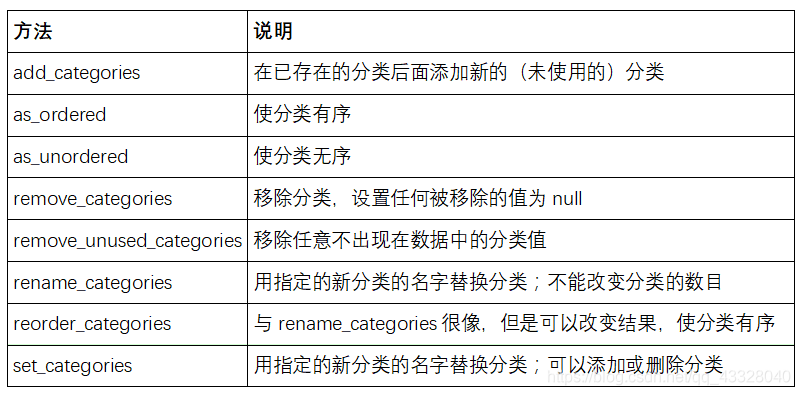
1.4分类方法
包含分类数据的Series有一些特殊的方法,类似于Series.str字符串方法。它还提供了快捷访问类别和代码的方法。看下面的Series:
s = pd.Series(['a', 'b', 'c', 'd'] * 2)
cat_s = s.astype('category')
cat_s
0    a
1    b
2    c
3    d
4    a
5    b
6    c
7    d
dtype: category
Categories (4, object): [a, b, c, d]
特殊属性cat提供了分类方法的入口:
cat_s.cat.codes
0    0
1    1
2    2
3    3
4    0
5    1
6    2
7    3
dtype: int8
cat_s.cat.categories
Index(['a', 'b', 'c', 'd'], dtype='object')
假设我们知道这个数据的实际分类集,超出了数据中的四个值。我们可以使用set_categories方法改变它们:
actual_categories = ['a', 'b', 'c', 'd', 'e']
cat_s2 = cat_s.cat.set_categories(actual_categories)
cat_s2
0    a
1    b
2    c
3    d
4    a
5    b
6    c
7    d
dtype: category
Categories (5, object): [a, b, c, d, e]
虽然数据看起来没变,但新的分类将反映在使用它们的操作中。例如,value_counts将遵循新的类别(如果存在):
cat_s.value_counts()
d    2
c    2
b    2
a    2
dtype: int64
cat_s2.value_counts()
d    2
c    2
b    2
a    2
e    0
dtype: int64
在大数据集中,分类经常作为节省内存和高性能的便捷工具。过滤完大DataFrame或Series之后,许多分类可能不会出现在数据中。我们可以使用remove_unused_categories方法删除没看到的分类:
cat_s3 = cat_s[cat_s.isin(['a', 'b'])]
cat_s3
0    a
1    b
4    a
5    b
dtype: category
Categories (4, object): [a, b, c, d]
cat_s3.cat.remove_unused_categories()
0    a
1    b
4    a
5    b
dtype: category
Categories (2, object): [a, b]
下表列出了可用的分类方法。
创建用于建模的虚拟变量
当你使用统计或机器学习工具时,通常会将分类数据转换为虚拟变量,也称为one-hot编码。这包括创建一个每一列都是不同类别DataFrame;这些列包含一个特定类别的出现次数,否则为0。
cat_s = pd.Series(['a', 'b', 'c', 'd'] * 2, dtype='category')
pandas.get_dummies函数可以转换这个分类数据为包含虚拟变量的DataFrame:
pd.get_dummies(cat_s)
| a | b | c | d | |
|---|---|---|---|---|
| 0 | 1 | 0 | 0 | 0 |
| 1 | 0 | 1 | 0 | 0 |
| 2 | 0 | 0 | 1 | 0 |
| 3 | 0 | 0 | 0 | 1 |
| 4 | 1 | 0 | 0 | 0 |
| 5 | 0 | 1 | 0 | 0 |
| 6 | 0 | 0 | 1 | 0 |
| 7 | 0 | 0 | 0 | 1 |
二.高阶GroupBy应用
管我们之前已经深度学习了Series和DataFrame的Groupby方法,还有一些方法也是很有用的。
2.1分组转换和’展开’GroupBy
我们在分组操作中学习了apply方法,进行转换。还有另一个transform方法,它与apply很像,但是对使用的函数有一定限制:
它可以产生向分组形状广播标量值
它可以产生一个和输入组形状相同的对象
它不能修改输入
来看一个简单的例子:
df = pd.DataFrame({'key': ['a', 'b', 'c'] * 4,
                   'value': np.arange(12.)})
df
| key | value | |
|---|---|---|
| 0 | a | 0.0 |
| 1 | b | 1.0 |
| 2 | c | 2.0 |
| 3 | a | 3.0 |
| 4 | b | 4.0 |
| 5 | c | 5.0 |
| 6 | a | 6.0 |
| 7 | b | 7.0 |
| 8 | c | 8.0 |
| 9 | a | 9.0 |
| 10 | b | 10.0 |
| 11 | c | 11.0 |
按’key’进行分组:
g = df.groupby('key').value
g.mean()
key
a    4.5
b    5.5
c    6.5
Name: value, dtype: float64
假设我们想产生一个和df[‘value’]形状相同的Series,但值替换为按’key’分组的平均值。我们可以传递函数lambda x: x.mean()进行转换:
g.transform(lambda x: x.mean())
0     4.5
1     5.5
2     6.5
3     4.5
4     5.5
5     6.5
6     4.5
7     5.5
8     6.5
9     4.5
10    5.5
11    6.5
Name: value, dtype: float64
对于内置的聚合函数,我们想GroupBy的agg方法一样传递一个字符串别名:
g.transform('mean')
0     4.5
1     5.5
2     6.5
3     4.5
4     5.5
5     6.5
6     4.5
7     5.5
8     6.5
9     4.5
10    5.5
11    6.5
Name: value, dtype: float64
与apply类似,transform的函数会返回Series,但是结果必须与输入大小相同。举个例子,我们可以用lambda函数将每个分组乘以2:
g.transform(lambda x: x * 2)
0      0.0
1      2.0
2      4.0
3      6.0
4      8.0
5     10.0
6     12.0
7     14.0
8     16.0
9     18.0
10    20.0
11    22.0
Name: value, dtype: float64
再举一个复杂的例子,我们可以计算每个分组的降序排名:
g.transform(lambda x: x.rank(ascending=False))
0     4.0
1     4.0
2     4.0
3     3.0
4     3.0
5     3.0
6     2.0
7     2.0
8     2.0
9     1.0
10    1.0
11    1.0
Name: value, dtype: float64
看一个由简单聚合构造的的分组转换函数:
def normalize(x):
    return (x - x.mean()) / x.std()
我们用transform或apply可以获得等价的结果:
g.transform(normalize)
0    -1.161895
1    -1.161895
2    -1.161895
3    -0.387298
4    -0.387298
5    -0.387298
6     0.387298
7     0.387298
8     0.387298
9     1.161895
10    1.161895
11    1.161895
Name: value, dtype: float64
g.apply(normalize)
0    -1.161895
1    -1.161895
2    -1.161895
3    -0.387298
4    -0.387298
5    -0.387298
6     0.387298
7     0.387298
8     0.387298
9     1.161895
10    1.161895
11    1.161895
Name: value, dtype: float64
内置的聚合函数,比如mean或sum,通常比apply函数快。这些函数在与transform一起使用时也会存在一个’快速通过’。这允许我们执行一个所谓的展开分组操作
g.transform('mean')
0     4.5
1     5.5
2     6.5
3     4.5
4     5.5
5     6.5
6     4.5
7     5.5
8     6.5
9     4.5
10    5.5
11    6.5
Name: value, dtype: float64
normalized = (df['value'] - g.transform('mean')) / g.transform('std')
normalized
0    -1.161895
1    -1.161895
2    -1.161895
3    -0.387298
4    -0.387298
5    -0.387298
6     0.387298
7     0.387298
8     0.387298
9     1.161895
10    1.161895
11    1.161895
Name: value, dtype: float64
解封分组操作可能包括多个分组聚合,但是矢量化操作还是会带来收益。
2.2分组的时间重新采样
对于时间序列数据,resample方法从语义上是一个基于内在时间的分组操作。下面是一个示例表:
N = 15
times = pd.date_range('2017-05-20 00:00', freq='1min', periods=N)
df = pd.DataFrame({'time': times,
                   'value': np.arange(N)})
df
| time | value | |
|---|---|---|
| 0 | 2017-05-20 00:00:00 | 0 |
| 1 | 2017-05-20 00:01:00 | 1 |
| 2 | 2017-05-20 00:02:00 | 2 |
| 3 | 2017-05-20 00:03:00 | 3 |
| 4 | 2017-05-20 00:04:00 | 4 |
| 5 | 2017-05-20 00:05:00 | 5 |
| 6 | 2017-05-20 00:06:00 | 6 |
| 7 | 2017-05-20 00:07:00 | 7 |
| 8 | 2017-05-20 00:08:00 | 8 |
| 9 | 2017-05-20 00:09:00 | 9 |
| 10 | 2017-05-20 00:10:00 | 10 |
| 11 | 2017-05-20 00:11:00 | 11 |
| 12 | 2017-05-20 00:12:00 | 12 |
| 13 | 2017-05-20 00:13:00 | 13 |
| 14 | 2017-05-20 00:14:00 | 14 |
这里,我们可以用time作为索引,然后重采样:
df.set_index('time').resample('5min').count()
| value | |
|---|---|
| time | |
| 2017-05-20 00:00:00 | 5 |
| 2017-05-20 00:05:00 | 5 |
| 2017-05-20 00:10:00 | 5 |
三.方法链技术
当对数据集进行一系列变换时,你可能发现创建的多个临时变量其实并没有在分析中用到。看下面的例子:
df = load_data()
df2 = df[df['col2'] < 0]
df2['col1_demeaned'] = df2['col1'] - df2['col1'].mean()
result = df2.groupby('key').col1_demeaned.std()
虽然这里没有使用真实的数据,这个例子却指出了一些新方法。首先,DataFrame.assign方法是一个df[k] = v形式的函数式的列分配方法。它不是就地修改对象,而是返回新的修改过的DataFrame。因此,下面的语句是等价的:
# Usual non-functional way
df2 = df.copy()
df2['k'] = v
# Functional assign way
df2 = df.assign(k=v)
原位赋值可能比使用assign更为快速,但是assign可以方便地进行链式编程:
result = (df2.assign(col1_demeaned=df2.col1 - df2.col2.mean())
          .groupby('key')
          .col1_demeaned.std())
我使用外括号,这样便于添加换行符。
使用链式编程时要注意,你可能会需要涉及临时对象。在前面的例子中,我们不能使用load_data的结果,直到它被赋值给临时变量df。为了这么做,assign和许多其它pandas函数可以接收类似函数的参数,即可调用参数。为了展示可调用对象,看一个前面例子的片段:
df = load_data()
df2 = df[df['col2'] < 0]
它可以重写为:
df = (load_data()[lambda x: x['col2'] < 0])
这里,load_data的结果没有赋值给某个变量,因此传递到[ ]的函数在这一步被绑定到了对象上。
我们可以把整个过程写为一个单链表达式:
result = (load_data()
          [lambda x: x.col2 < 0]
          .assign(col1_demeaned=lambda x: x.col1 - x.col1.mean())
          .groupby('key')
          .col1_demeaned.std())
是否将代码写成这种形式只是习惯而已,将它分开成若干步可以提高可读性。
3.1 pipe(管道)方法
你可以用Python内置的pandas函数和方法,用带有可调用对象的链式编程做许多工作。但是,有时你需要使用自己的函数,或是第三方库的函数。这时就要用到管道方法。
看下面的函数调用:
a = f(df, arg1=v1)
b = g(a, v2, arg3=v3)
c = h(b, arg4=v4)
当使用接收、返回Series或DataFrame对象的函数式,你可以调用pipe将其重写:
result = (df.pipe(f, arg1=v1)
          .pipe(g, v2, arg3=v3)
          .pipe(h, arg4=v4))
f(df)和df.pipe(f)是等价的,但是pipe使得链式声明更容易。
将操作的序列泛化成可复用的函数是pipe方法的一个潜在用途。作为实例,让我们考虑从一列中减去分组平均值:
g = df.groupby(['key1', 'key2'])
df['col1'] = df['col1'] - g.transform('mean')
假设你想转换多列,并修改分组的键。另外,你想用链式编程做这个转换。下面就是一个方法:
def group_demean(df, by, cols):
    result = df.copy()
    g = df.groupby(by)
    for c in cols:
        result[c] = df[c] - g[c].transform('mean')
    return result
然后可以写为:
result = (df[df.col1 < 0]
          .pipe(group_demean, ['key1', 'key2'], ['col1']))