【Spark MLlib】（七）Spark MLlib 中随机森林 RF（Random Forest）源码深度解析

一、背景

使用 Spark 机器学习库来做机器学习工作，可以说是非常的简单，通常只需要在对原始数据进行处理后，然后直接调用相应的 API 就可以实现。但是要想选择合适的算法，高效准确地对数据进行分析，可能还需要深入了解下算法原理，以及相应 Spark MLlib API 实现的参数的意义。

目前，Spark MLlib 中实现了 tree 相关的算法，决策树 DT（DecisionTree），随机森林 RF（Random Forest），GBDT（Gradient Boosting Decision Tree），其基础都是RF，DT 是 RF 一棵树时的情况，而 GBDT 则是循环构建DT，GBDT与DT的代码是非常简单明了的，本文会对 Random Forest 的源码进行分析，介绍 Spark 在实现过程中使用的一些技巧。

二、决策树与随机森林

首先我们来对决策树和随机森林进行简单的了解：

决策树 GBDT-Decision Tree(DT)

• 关键问题
  • 节点分裂：使用的特征及阈值
    • 特征选取：最小均方差、信息增益（ID3）、信息增益率（C4.5）
    • 阈值：从特征值中选取、等步长选取最大最小值之间的值
  • 叶子节点的值：叶子所属数据的均值（回归）、对应类别（分类）
  • 截止条件：达到叶子节点数上限、继续划分无法使误差减小

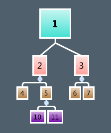
在决策树的训练中，如上图所示，就是从根节点开始，不断的分裂，直到触发截止条件，在节点的分裂过程中要解决的问题其实就两个：

• 分裂点：一般就是遍历所有特征的所有特征值，选取impurity最大的分成左右孩子节点，impurity的选取有信息熵（分类），最小均方差（回归）等方法
• 预测值：一般取当前最多的class（分类）或者取均值（回归）

随机森林

随机森林就是构建多棵决策树投票，在构建多棵树过程中，引入随机性，一般体现在两个方面，一是每棵树使用的样本进行随机抽样，分为有放回和无放回抽样。二是对每棵树使用的特征集进行抽样，使用部分特征训练。

在训练过程中，如果单机内存能放下所有样本，可以用多线程同时训练多棵树，树之间的训练互不影响。

三、Spark RF 优化策略

Spark MLlib 在实现随机森林(Random Forest) 时，我们可以使用一些优化技巧，提高训练效率。

3.1 逐层训练

当样本量过大，单机无法容纳时，只能采用分布式的训练方法，数据是在集群中的多台机器存放，如果按照单机的方法，每棵树完全独立访问样本数据，则样本数据的访问次数为数的个数k*每棵树的节点数N，相当于深度遍历。在spark的实现中，因为数据存放在不同的机器上，频繁的访问数据效率非常低，因此采用广度遍历的方法，每次构造所有树的一层，例如如果要训练10棵树，第一次构造所有树的第一层根节点，第二次构造所有深度为2的节点，以此类推，这样访问数据的次数降为树的最大深度，大大减少了机器之间的通信，提高训练效率。

3.2 样本抽样

当样本存在连续特征时，其可能的取值可能是无限的，存储其可能出现的值占用较大空间，因此spark对样本进行了抽样，抽样数量

val requiredSamples = math.max(metadata.maxBins * metadata.maxBins, 10000)

最少抽样1万条，当然这样会降低模型精度。

3.3 特征装箱

其实没什么神秘的，每个离散特征值(对于连续特征，先离散化)称为一个Split，上下限[lowSplit, highSplit]组成一个bin，也就是特征装箱，默认的maxBins是32。对于连续特征，离散化时的bin的个数就是maxBins，采用等频离散化；对于有序的离散特征，bin的个数是特征值个数+1；对于无序离散特征，bin的个数是2^(M-1)-1，M是特征值个数。

四、源码分析

从官方给出的分类demo开始，逐层分析其实现

4.1 训练数据的解析

主要是LabelPoint的构造，官方demo中要求训练数据是LibSVM格式的

parsed.map { case (label, indices, values) =>
      LabeledPoint(label, Vectors.sparse(d, indices, values))
    }

可以看到LabelPoint有两个成员，第一个是样本label，第二个是稀疏向量SparseVector，d是其size，在这里其实是特征数，indices是实际非0特征的index，values里面是实际的特征值，这里需要注意的是，SVN格式的特征index是从0开始的，这里进行了-1，变成从0开始了。

4.2 demo中训练参数说明

官方demo中只设置了部分参数

val model = RandomForest.trainClassifier(trainingData, numClasses, categoricalFeaturesInfo,
      numTrees, featureSubsetStrategy, impurity, maxDepth, maxBins)

• categoricalFeaturesInfo：Map[Int, Int]，key是特征的index，value为特征值的个数（或者说几种），这里值得注意的是，因为LabelPoint中进行了index-1的变换，这个里面的key也需要-1（参见后面metadata的numBins的计算）。例如性别这个特征在样本中的index为1，特征值男/女两种，则0->2
• featureSubsetStrategy：特征子集的抽取方法，支持”auto”, “all”, “sqrt”, “log2”, “onethird”
• impurity：不纯度，其实就是节点分裂时的衡量准则，例如信息熵，均方差等，这里支持三种，gini（基尼指数），entripy（信息熵），variance（均方差）
• maxDepth：树的最大深度
• maxBins：最大装箱数，或者说是特征的最大可能切分数+1。这个值必须大于等于最大的离散特征值数

4.3 参数封装

Spark MLlib 根据用户提供的参数值，进行实际训练参数的计算，并且将这些参数封装成类，方便传递。

4.3.1 Strategy

class Strategy @Since("1.3.0") (
    @Since("1.0.0") @BeanProperty var algo: Algo,
    @Since("1.0.0") @BeanProperty var impurity: Impurity,
    @Since("1.0.0") @BeanProperty var maxDepth: Int,
    @Since("1.2.0") @BeanProperty var numClasses: Int = 2,
    @Since("1.0.0") @BeanProperty var maxBins: Int = 32,
    @Since("1.0.0") @BeanProperty var quantileCalculationStrategy: QuantileStrategy = Sort,
    @Since("1.0.0") @BeanProperty var categoricalFeaturesInfo: Map[Int, Int] = Map[Int, Int](),
    @Since("1.2.0") @BeanProperty var minInstancesPerNode: Int = 1,
    @Since("1.2.0") @BeanProperty var minInfoGain: Double = 0.0,
    @Since("1.0.0") @BeanProperty var maxMemoryInMB: Int = 256,
    @Since("1.2.0") @BeanProperty var subsamplingRate: Double = 1,
    @Since("1.2.0") @BeanProperty var useNodeIdCache: Boolean = false,
    @Since("1.2.0") @BeanProperty var checkpointInterval: Int = 10)

• algo：classification/regression
• quantileCalculationStrategy：分位点（Split）策略，目前只支持Sort，对于连续型特征值，先把特征值进行排序，然后按次序取分位点。从代码中可以看到原来可能打算实现的MinMax和ApproxHist目前没有实现。
• minInstancesPerNode：每个树节点中最小的样本数，低于将不再对节点进行分裂，默认为1，可作为提前截止条件
• minInfoGain：最小增益，节点分裂后的增益如果小于它，将不再进行分裂，可作为提前截止条件
• subsamplingRate：样本抽样率，默认为1，每棵树都使用全部样本
• isMulticlassClassification：是否是多分类，判断条件为Classification 并且类别>2
• isMulticlassWithCategoricalFeatures：是否是带类别特征的多分类，判断条件再上面的基础上加categoricalFeaturesInfo的size大于0

4.3.2. metadata

在buildMetadata中根据strategy计算得到DecisionTreeMetadata的参数。

class DecisionTreeMetadata(
    val numFeatures: Int,
    val numExamples: Long,
    val numClasses: Int,
    val maxBins: Int,
    val featureArity: Map[Int, Int],
    val unorderedFeatures: Set[Int],
    val numBins: Array[Int],
    val impurity: Impurity,
    val quantileStrategy: QuantileStrategy,
    val maxDepth: Int,
    val minInstancesPerNode: Int,
    val minInfoGain: Double,
    val numTrees: Int,
    val numFeaturesPerNode: Int)

部分参数同Strategy，对额外参数和区别说明

• numClasses：如为Regression，设为0
• maxPossibleBins：取maxBins和样本数量中较小的；必须大于categoricalFeaturesInfo中的最大的离散特征值数
• numBins：所有特征及其特征值数，Int数组，维数是特征数，默认大小是maxPossibleBins。对于连续特征，其值就是默认值maxPossibleBins。对于离散特征，如为二分类或回归，此处将categoricalFeaturesInfo中的key特征index作为数组index，value特征个数写入数组中（这里有疑问，SVM格式的index是从1开始的，因此对numBins的index应该是categoricalFeaturesInfo的key-1，这里没有-1，当最大值等于maxBins的时候访问数组会抛异常）；如果是多分类，先计算其当做当UnorderedFeature（无序的离散特征）的bin，如果个数小于等于maxPossibleBins，会被当成UnorderedFeature，否则被当成orderedFeatures（为了防止计算指数溢出，实际是把maxPossibleBins取log与特征数比较），因为UnorderedFeature的bin是比较大，这里限制了其特征值不能太多，这里仅仅根据特征值的特殊决定是否是ordered，不太好。每个split要将所有特征值分成2部分，bin的数量也就是2split，因此bin的个数是2(2^(M-1)-1)
• numFeaturesPerNode：由featureSubsetStrategy决定，如果为“auto”，且为单棵树，则使用全部特征；如为多棵树，分类则是sqrt，回归为1/3；也可以自己指定，支持”all”, “sqrt”, “log2”, “onethird”。

五、特征处理

这部分主要在 DecisionTree.scala 的 findSplitsBins 函数，将所有特征封装成Split，然后装箱Bin。首先对split和bin的结构进行说明。

5.1 数据结构

5.1.1 Split

class Split(
    @Since("1.0.0") feature: Int,
    @Since("1.0.0") threshold: Double,
    @Since("1.0.0") featureType: FeatureType,
    @Since("1.0.0") categories: List[Double])

• feature：特征id
• threshold：阈值
• featureType：连续特征（Continuous）/离散特征（Categorical）
• categories：离散特征值数组，离散特征使用。放着此split中所有特征值

5.1.2 Bin

class Bin(
    lowSplit: Split, 
    highSplit: Split, 
    featureType: FeatureType, 
    category: Double)

• lowSplit/highSplit：上下界
• featureType：连续特征（Continuous）/离散特征（Categorical）
• category：离散特征的特征值

5.2 连续特征处理

5.2.1 抽样

val continuousFeatures = Range(0, numFeatures).filter(metadata.isContinuous)
val sampledInput = if (continuousFeatures.nonEmpty) {
      // Calculate the number of samples for approximate quantile calculation.
      val requiredSamples = math.max(metadata.maxBins * metadata.maxBins, 10000)
      val fraction = if (requiredSamples < metadata.numExamples) {
        requiredSamples.toDouble / metadata.numExamples
      } else {
        1.0
      }
      logDebug("fraction of data used for calculating quantiles = " + fraction)
      input.sample(withReplacement = false, fraction, new XORShiftRandom().nextInt())
    } else {
      input.sparkContext.emptyRDD[LabeledPoint]
    }

首先筛选出连续特征集，然后计算抽样数量，抽样比例，然后无放回样本抽样；如果没有连续特征，则为空RDD。

5.2.2 计算Split

metadata.quantileStrategy match {
      case Sort =>
        findSplitsBinsBySorting(sampledInput, metadata, continuousFeatures)
      case MinMax =>
        throw new UnsupportedOperationException("minmax not supported yet.")
      case ApproxHist =>
        throw new UnsupportedOperationException("approximate histogram not supported yet.")
    }

分位点策略，这里只实现了Sort这一种，前文有说明，下面的计算在findSplitsBinsBySorting函数中，入参是抽样样本集，metadata和连续特征集（里面是特征id，从0开始，见LabelPoint的构造）

val continuousSplits = {
    // reduce the parallelism for split computations when there are less
    // continuous features than input partitions. this prevents tasks from
    // being spun up that will definitely do no work.
    val numPartitions = math.min(continuousFeatures.length,input.partitions.length)
    input.flatMap(point => continuousFeatures.map(idx =>  (idx,point.features(idx))))
         .groupByKey(numPartitions)
         .map { case (k, v) => findSplits(k, v) }
         .collectAsMap()
    }

特征id为key，value是样本对应的该特征下的所有特征值，传给findSplits函数，其中又调用了findSplitsForContinuousFeature函数获得连续特征的Split，入参为样本，metadata和特征id

def findSplitsForContinuousFeature(
      featureSamples: Array[Double], 
      metadata: DecisionTreeMetadata,
      featureIndex: Int): Array[Double] = {
    require(metadata.isContinuous(featureIndex),
      "findSplitsForContinuousFeature can only be used to find splits for a continuous feature.")

    val splits = {
    //连续特征的split是numBins-1
      val numSplits = metadata.numSplits(featureIndex)
    //统计所有特征值其出现的次数
      // get count for each distinct value
      val valueCountMap = featureSamples.foldLeft(Map.empty[Double, Int]) { (m, x) =>
        m + ((x, m.getOrElse(x, 0) + 1))
      }
      //按特征值排序
      // sort distinct values
      val valueCounts = valueCountMap.toSeq.sortBy(_._1).toArray

      // if possible splits is not enough or just enough, just return all possible splits
      val possibleSplits = valueCounts.length
      if (possibleSplits <= numSplits) {
        valueCounts.map(_._1)
      } else {
      //等频离散化
        // stride between splits
        val stride: Double = featureSamples.length.toDouble / (numSplits + 1)
        logDebug("stride = " + stride)

        // iterate `valueCount` to find splits
        val splitsBuilder = Array.newBuilder[Double]
        var index = 1
        // currentCount: sum of counts of values that have been visited
        var currentCount = valueCounts(0)._2
        // targetCount: target value for `currentCount`.
        // If `currentCount` is closest value to `targetCount`,
        // then current value is a split threshold.
        // After finding a split threshold, `targetCount` is added by stride.
        var targetCount = stride
        while (index < valueCounts.length) {
          val previousCount = currentCount
          currentCount += valueCounts(index)._2
          val previousGap = math.abs(previousCount - targetCount)
          val currentGap = math.abs(currentCount - targetCount)
          // If adding count of current value to currentCount
          // makes the gap between currentCount and targetCount smaller,
          // previous value is a split threshold.
          //每次步进targetCount个样本，取上一个特征值与下一个特征值gap较小的
          if (previousGap < currentGap) {
            splitsBuilder += valueCounts(index - 1)._1
            targetCount += stride
          }
          index += 1
        }

        splitsBuilder.result()
      }
    }

    // TODO: Do not fail; just ignore the useless feature.
    assert(splits.length > 0,
      s"DecisionTree could not handle feature $featureIndex since it had only 1 unique value." +
        "  Please remove this feature and then try again.")

    // the split metadata must be updated on the driver

    splits
  }

在构造split的过程中，如果统计到的值的个数possibleSplits 还不如你设置的numSplits多，那么所有的值都作为分割点；否则，用等频分隔法，首先计算分隔步长stride，然后再循环中每次累加到targetCount中，作为理想分割点，但是理想分割点可能会包含的特征值过多，想取一个里理想分割点尽量近的特征值，例如，理想分割点是100，落在特征值fc里，但是当前特征值里面有30个样本，而前一个特征值fp只有5个样本，因此我们如果取fc作为split，则当前区间实际多25个样本，如果取fp，则少5个样本，显然取fp更为合理。

具体到代码实现，在if判断里步进stride个样本，累加在targetCount中。while循环逐次把每个特征值的个数加到currentCount里，计算前一次previousCount和这次currentCount到targetCount的距离，有3种情况，一种是pre和cur都在target左边，肯定是cur小，继续循环，进入第二种情况；第二种一左一右，如果pre小，肯定是pre是最好的分割点，如果cur还是小，继续循环步进，进入第三种情况；第三种就是都在右边，显然是pre小。因此if的判断条件pre<cur，只要满足肯定就是split。整体下来的效果就能找到离target最近的一个特征值。
findSplits函数使用本函数得到的离散化点作为threshold，构造Split。

val splits = {
    val featureSplits = findSplitsForContinuousFeature(
          featureSamples.toArray,
          metadata,
          featureIndex)
    logDebug(s"featureIndex = $featureIndex, numSplits = ${featureSplits.length}")

    featureSplits.map(threshold => new Split(featureIndex, threshold, Continuous, Nil))
}

这样就得到了连续特征所有的Split。

5.2.3 计算bin

得到splits后，即可类似滑窗得到bin的上下界，构造bins

val bins = {
    val lowSplit = new DummyLowSplit(featureIndex, Continuous)
    val highSplit = new DummyHighSplit(featureIndex, Continuous)

    // tack the dummy splits on either side of the computed splits
    val allSplits = lowSplit +: splits.toSeq :+ highSplit

    // slide across the split points pairwise to allocate the bins
    allSplits.sliding(2).map {
         case Seq(left, right) => new Bin(left, right, Continuous, Double.MinValue)
    }.toArray
}

在计算splits的时候，个数是bin的个数减1，这里加上第一个DummyLowSplit（threshold是Double.MinValue)，和最后一个DummyHighSplit（threshold是Double.MaxValue)构造的bin，恰好个数是numBins中的个数。

5.3 离散特征

bin的主要作用其实就是用来做连续特征离散化，离散特征是用不着的。
对有序离散特征而言，其split直接用特征值表征，因此这里的splits和bins都是空的Array。
对于无序离散特征而言，其split是特征值的组合，不是简单的上下界比较关系，bin是空Array，而split需要计算。

5.3.1 split

// Unordered features
// 2^(maxFeatureValue - 1) - 1 combinations
val featureArity = metadata.featureArity(i)
val split = Range(0, metadata.numSplits(i)).map { splitIndex =>
    val categories = extractMultiClassCategories(splitIndex + 1, featureArity)
    new Split(i, Double.MinValue, Categorical, categories)
}

featureArity来自参数categoricalFeaturesInfo中设置的离散特征的特征值数。
metadata.numSplits是吧numBins中的数量/2，相当于返回了2^(M-1)-1，M是特征值数。
调用extractMultiClassCategories函数，入参是1到2^(M-1)和特征数M。

/**
   * Nested method to extract list of eligible categories given an index. It extracts the
   * position of ones in a binary representation of the input. If binary
   * representation of an number is 01101 (13), the output list should (3.0, 2.0,
   * 0.0). The maxFeatureValue depict the number of rightmost digits that will be tested for ones.
   */
def extractMultiClassCategories(
     input: Int,
     maxFeatureValue: Int): List[Double] = {
    var categories = List[Double]()
    var j = 0
    var bitShiftedInput = input
    while (j < maxFeatureValue) {
      if (bitShiftedInput % 2 != 0) {
        // updating the list of categories.
        categories = j.toDouble :: categories
      }
      // Right shift by one
      bitShiftedInput = bitShiftedInput >> 1
      j += 1
    }
    categories
}

如注释所述，这个函数返回给定的input的二进制表示中1的index，这里实际返回的是特征的组合。这里可以了解一下组合数。

六、样本处理

将输入样本LabelPoint与上述特征进一步封装，方便后面进行分区统计。

6.1 TreePoint

构造TreePoint的过程，是一系列函数的调用链，我们逐层分析。

val treeInput = TreePoint.convertToTreeRDD(retaggedInput, bins, metadata)

RandomForest.scala中将输入转化成TreePoint的rdd，调用convertToTreeRDD函数 。

def convertToTreeRDD(
    input: RDD[LabeledPoint],
    bins: Array[Array[Bin]],
    metadata: DecisionTreeMetadata): RDD[TreePoint] = {
    // Construct arrays for featureArity for efficiency in the inner loop.
    val featureArity: Array[Int] = new Array[Int](metadata.numFeatures)
    var featureIndex = 0
    while (featureIndex < metadata.numFeatures) {
      featureArity(featureIndex) = metadata.featureArity.getOrElse(featureIndex, 0)
      featureIndex += 1
    }
    input.map { x =>
      TreePoint.labeledPointToTreePoint(x, bins, featureArity)
    }
  }

convertToTreeRDD函数的入参input是所有样本，bins是二维数组，第一维是特征，第二维是特征的Bin数组。函数首先计算每个特征的特征数量，放在featureArity中，如果是连续特征，设为0。对每个样本调用labeledPointToTreePoint函数，构造TreePoint。

private def labeledPointToTreePoint(
      labeledPoint: LabeledPoint,
      bins: Array[Array[Bin]],
      featureArity: Array[Int]): TreePoint = {
    val numFeatures = labeledPoint.features.size
    val arr = new Array[Int](numFeatures)
    var featureIndex = 0
    while (featureIndex < numFeatures) {
      arr(featureIndex) = findBin(featureIndex, labeledPoint, featureArity(featureIndex),
        bins)
      featureIndex += 1
    }
    new TreePoint(labeledPoint.label, arr)
  }

labeledPointToTreePoint计算每个样本的所有特征对应的特征值属于哪个bin，放在在arr数组中；如果是连续特征，存放的实际是binIndex，或者说是第几个bin；如果是离散特征，直接featureValue.toInt，这其实暗示着，对有序离散值，其编码只能是[0,featureArity - 1]，闭区间，其后的部分逻辑也依赖于这个假设。这部分是在findBin函数中完成的，这里不再赘述。

我们在这里把TreePoint的成员再罗列一下，方便查阅

class TreePoint(val label: Double, val binnedFeatures: Array[Int])

这里是把每个样本从LabelPoint转换成TreePoint，label就是样本label，binnedFeatures就是上述的arr数组。

6.2 BaggedPoint

同理构造BaggedPoint的过程，也是一系列函数的调用链，我们逐层分析。

val withReplacement = if (numTrees > 1) true else false
val baggedInput = BaggedPoint.convertToBaggedRDD(treeInput,
          strategy.subsamplingRate, numTrees,
          withReplacement, seed).persist(StorageLevel.MEMORY_AND_DISK)

这里同时对样本进行了抽样，如果树个数大于1，就有放回抽样，否则无放回抽样，调用convertToTreeRDD函数将TreePoint转化成BaggedPoint的rdd 。

/**
   * Convert an input dataset into its BaggedPoint representation,
   * choosing subsamplingRate counts for each instance.
   * Each subsamplingRate has the same number of instances as the original dataset,
   * and is created by subsampling without replacement.
   * @param input Input dataset.
   * @param subsamplingRate Fraction of the training data used for learning decision tree.
   * @param numSubsamples Number of subsamples of this RDD to take.
   * @param withReplacement Sampling with/without replacement.
   * @param seed Random seed.
   * @return BaggedPoint dataset representation.
   */
  def convertToBaggedRDD[Datum] (
      input: RDD[Datum],
      subsamplingRate: Double,
      numSubsamples: Int,
      withReplacement: Boolean,
      seed: Long = Utils.random.nextLong()): RDD[BaggedPoint[Datum]] = {
    if (withReplacement) {
      convertToBaggedRDDSamplingWithReplacement(input, subsamplingRate, numSubsamples, seed)
    } else {
      if (numSubsamples == 1 && subsamplingRate == 1.0) {
        convertToBaggedRDDWithoutSampling(input)
      } else {
        convertToBaggedRDDSamplingWithoutReplacement(input, subsamplingRate, numSubsamples, seed)
      }
    }
  }

根据有放回还是无放回，或者不抽样分别调用相应函数。无放回抽样 。

def convertToBaggedRDDSamplingWithoutReplacement[Datum] (
      input: RDD[Datum],
      subsamplingRate: Double,
      numSubsamples: Int,
      seed: Long): RDD[BaggedPoint[Datum]] = {
    //对每个partition独立抽样
    input.mapPartitionsWithIndex { (partitionIndex, instances) =>
      // Use random seed = seed + partitionIndex + 1 to make generation reproducible.
      val rng = new XORShiftRandom
      rng.setSeed(seed + partitionIndex + 1)
      instances.map { instance =>
      //对每条样本进行numSubsamples（实际是树的个数）次抽样，
      //一次将本条样本在所有树中是否会被抽取都获得，牺牲空间减少访问数据次数
        val subsampleWeights = new Array[Double](numSubsamples)
        var subsampleIndex = 0
        while (subsampleIndex < numSubsamples) {
          val x = rng.nextDouble()
          //无放回抽样，只需要决定本样本是否被抽取，被抽取就是1，没有就是0
          subsampleWeights(subsampleIndex) = {
            if (x < subsamplingRate) 1.0 else 0.0
          }
          subsampleIndex += 1
        }
        new BaggedPoint(instance, subsampleWeights)
      }
    }
  }

有放回抽样

def convertToBaggedRDDSamplingWithReplacement[Datum] (
      input: RDD[Datum],
      subsample: Double,
      numSubsamples: Int,
      seed: Long): RDD[BaggedPoint[Datum]] = {
    input.mapPartitionsWithIndex { (partitionIndex, instances) =>
      // Use random seed = seed + partitionIndex + 1 to make generation reproducible.
      val poisson = new PoissonDistribution(subsample)
      poisson.reseedRandomGenerator(seed + partitionIndex + 1)
      instances.map { instance =>
        val subsampleWeights = new Array[Double](numSubsamples)
        var subsampleIndex = 0
        while (subsampleIndex < numSubsamples) {
        //与无放回抽样对比，这里用泊松抽样返回的是样本被抽取的次数，
        //可能大于1，而无放回是0/1，也可认为是被抽取的次数
          subsampleWeights(subsampleIndex) = poisson.sample()
          subsampleIndex += 1
        }
        new BaggedPoint(instance, subsampleWeights)
      }
    }
  }

不抽样，或者说抽样率为1

def convertToBaggedRDDWithoutSampling[Datum] (
      input: RDD[Datum]): RDD[BaggedPoint[Datum]] = {
    input.map(datum => new BaggedPoint(datum, Array(1.0)))
  }

这里再啰嗦的罗列下BaggedPoint

class BaggedPoint[Datum](
    val datum: Datum, 
    val subsampleWeights: Array[Double])

datum是TreePoint，subsampleWeights是数组，维数等于numberTrees，每个值是样本在每棵树中被抽取的次数。

至此，Random Forest的初始化工作已经完成。

timer.stop("init")

七、随机森林训练

7.1 数据结构

7.1.1 Node

树中的每个节点是一个Node结构

class Node @Since("1.2.0") (
    @Since("1.0.0") val id: Int,
    @Since("1.0.0") var predict: Predict,
    @Since("1.2.0") var impurity: Double,
    @Since("1.0.0") var isLeaf: Boolean,
    @Since("1.0.0") var split: Option[Split],
    @Since("1.0.0") var leftNode: Option[Node],
    @Since("1.0.0") var rightNode: Option[Node],
    @Since("1.0.0") var stats: Option[InformationGainStats])

emptyNode，只初始化nodeIndex，其他都是默认值

def emptyNode(nodeIndex: Int): Node = 
    new Node(nodeIndex, new Predict(Double.MinValue),
    -1.0, false, None, None, None, None)

根据node的id，计算孩子节点的id

   * Return the index of the left child of this node.
   */
  def leftChildIndex(nodeIndex: Int): Int = nodeIndex << 1

  /**
   * Return the index of the right child of this node.
   */
  def rightChildIndex(nodeIndex: Int): Int = (nodeIndex << 1) + 1

左孩子节点就是当前id * 2，右孩子是id * 2+1。

7.1.2 Entropy

7.1.2.1 Entropy

Entropy是个Object，里面最重要的是calculate函数 。

/**
   * :: DeveloperApi ::
   * information calculation for multiclass classification
   * @param counts Array[Double] with counts for each label
   * @param totalCount sum of counts for all labels
   * @return information value, or 0 if totalCount = 0
   */
  @Since("1.1.0")
  @DeveloperApi
  override def calculate(counts: Array[Double], totalCount: Double): Double = {
    if (totalCount == 0) {
      return 0
    }
    val numClasses = counts.length
    var impurity = 0.0
    var classIndex = 0
    while (classIndex < numClasses) {
      val classCount = counts(classIndex)
      if (classCount != 0) {
        val freq = classCount / totalCount
        impurity -= freq * log2(freq)
      }
      classIndex += 1
    }
    impurity
  }

未持完续 …