建立一个逻辑回归模型来预测一个学生是否被大学录取。假设你是一个大学管理员,你想根据两次考试的结果
来决定每个申请人的录取机会,你有以前申请人的历史数据,你可以用它作为逻辑回归的训练集。对于每一个培训
例子,有两个考试的申请人的分数和录取决定,为了做到这一点,建立一个分类模型,根据考试成绩估计入学概率。
导入数据,并读取数据
import numpy as np
import pandas as pd
import matplotlib.pyplot as plt
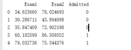
pdData=pd.read_csv("LogiReg_data.txt",header=None,names=['Exam1','Exam2','Admitted'])
print(pdData.head())
画图:
import numpy as np
import pandas as pd
import matplotlib.pyplot as plt

pdData=pd.read_csv("LogiReg_data.txt",header=None,names=['Exam1','Exam2','Admitted'])
# print(pdData.head())
# print(pdData.shape)

#画图
positive=pdData[pdData["Admitted"]==1]
negative=pdData[pdData["Admitted"]==0]

fig,ax=plt.subplots(figsize=(10,5))#指定画图域
#散点图
ax.scatter(positive['Exam1'],positive["Exam2"],s=30,c='b',marker='o',label="Admitted")
ax.scatter(negative['Exam1'],negative["Exam2"],s=30,c='r',marker='x',label="Not Admitted")
ax.legend()
ax.set_xlabel("Exam1 Score")
ax.set_ylabel("Exam2 Score")
plt.show()
The logistic regression
目标:建立分类器(求解出三个参数Θ0,Θ1,Θ2)
设定阈值,根据阈值判断录取结果
要完成的模块:
- sigmoid:映射到概率的函数
- model:返回预测结果值
- cost:根据参数计算损失
- gradient:计算每个参数的梯度方向
- descent:进行参数更新
- accuracy:计算精度
sigmoid函数:

def sigmoid(z):
    return 1/(1+np.exp(-z))
损失函数

#预测函数
def model(X,theta):
    return sigmoid(np.dot(X,theta.T))

pdData.insert(0,"Ones",1)#加入一列
orig_data=pdData.as_matrix()
cols=orig_data.shape[1]
X=orig_data[:,0:cols-1]
y=orig_data[:,cols-1:cols]

theta=np.zeros([1,3])
#print(X)
#print(y)
#print(theta)

def cost(X,y,theta):
    left=np.multiply(-y,np.log(model(X,theta)))
    right=np.multiply(1-y,np.log(1-model(X,theta)))
    return np.sum(left-right)/len(X)
计算梯度:

def gradient(X,y,theta):
    grad=np.zeros(theta.shape)
    error=(model(X,theta)-y).ravel()
    for i in range(len(theta.ravel())):
        term=np.multiply(error,X[:,j])
        grad[0,j]=np.sum(term)/len(X)
    return grad
Gradient descent
比较3种不同梯度下降方法:

#完整代码:
"""
建立一个逻辑回归模型来预测一个学生是否被大学录取。假设你是一个大学管理员,你想根据两次考试的结果
来决定每个申请人的录取机会,你有以前申请人的历史数据,你可以用它作为逻辑回归的训练集。对于每一个培训
例子,有两个考试的申请人的分数和录取决定,为了做到这一点,建立一个分类模型,根据考试成绩估计入学概率

"""

import numpy as np
import pandas as pd
import matplotlib.pyplot as plt

pdData=pd.read_csv("LogiReg_data.txt",header=None,names=['Exam1','Exam2','Admitted'])
# print(pdData.head())
# print(pdData.shape)

#画图
positive=pdData[pdData["Admitted"]==1]
negative=pdData[pdData["Admitted"]==0]

fig,ax=plt.subplots(figsize=(10,5))#指定画图域
#散点图
ax.scatter(positive['Exam1'],positive["Exam2"],s=30,c='b',marker='o',label="Admitted")
ax.scatter(negative['Exam1'],negative["Exam2"],s=30,c='r',marker='x',label="Not Admitted")
ax.legend()
ax.set_xlabel("Exam1 Score")
ax.set_ylabel("Exam2 Score")
#plt.show()


def sigmoid(z):
    return 1/(1+np.exp(-z))

#预测函数
def model(X,theta):
    return sigmoid(np.dot(X,theta.T))

pdData.insert(0,"Ones",1)#加入一列
orig_data=pdData.as_matrix()
cols=orig_data.shape[1]
X=orig_data[:,0:cols-1]
y=orig_data[:,cols-1:cols]

theta=np.zeros([1,3])
#print(X)
#print(y)
#print(theta)

def cost(X,y,theta):
    left=np.multiply(-y,np.log(model(X,theta)))
    right=np.multiply(1-y,np.log(1-model(X,theta)))
    return np.sum(left-right)/len(X)

print(cost(X,y,theta))


def gradient(X,y,theta):
    grad=np.zeros(theta.shape)
    error=(model(X,theta)-y).ravel()
    for j in range(len(theta.ravel())):
        term=np.multiply(error,X[:,j])
        grad[0,j]=np.sum(term)/len(X)
    return grad


STOP_ITER=0#根据迭代次数停止
STOP_COST=1#根据迭代损失停止
STOP_GRAD=2#根据梯度

def stopCriterion(type,value,threshold):
    #设定三种不同停止策略
    if type==STOP_ITER:
        return value>threshold
    elif type==STOP_COST:
        return abs(value[-1]-value[-2])<threshold
    elif type==STOP_GRAD:
        return np.linalg.norm(value)<threshold

import numpy.random
#洗牌,打乱数据顺序
def shuffleData(data):
    np.random.shuffle(data)
    cols=data.shape[1]
    X=data[:,0:cols-1]
    y=data[:,cols-1:]
    return X,y

import time

def descent(data,theta,batchSize,stopType,thresh,alpha):
    #梯度下降求解
    init_time=time.time()
    i=0#迭代次数
    k=0#batch
    X,y=shuffleData(data)
    grad=np.zeros(theta.shape)#计算的梯度
    costs=[cost(X,y,theta)]#损失值

    while True:
        grad=gradient(X[k:k+batchSize],y[k:k+batchSize],theta)
        k+=batchSize#取batch数量个数据
        if k>=n:
            k=0
            X,y=shuffleData(data)#重新洗牌
        theta=theta-alpha*grad#参数更新
        costs.append(cost(X,y,theta))#计算新的损失
        i+=1

        if stopType==STOP_ITER:
            value=1
        elif stopType==STOP_COST:
            value=costs
        elif stopType==STOP_GRAD:
            value=grad
        if stopCriterion(stopType,value,thresh):
            break
    return theta,i-1,costs,grad,time.time()-init_time

def runExpe(data,theta,batchSize,stopType,thresh,alpha):
    theta,iter,costs,grad,dur=descent(data,theta,batchSize,stopType,thresh,alpha
                                      )
    name="Orignal" if(data[:,1]>2).sum()>1 else "Scaled"
    name+= " data - learning rate:{}=".format(alpha)
    if batchSize==n:strDescType="Gradient"
    elif batchSize==1:strDescType="Stochastic"
    else:strDescType="Mini-batch({})".format(batchSize)
    name+=strDescType+" desent - Stop:"
    if stopType ==STOP_ITER:strStop="{}iterations".format(thresh)
    elif stopType==stopType==STOP_COST:strStop="costs change<{}".format(thresh)
    else:strStop="gradient norm<{}".format(thresh)
    name+=strStop
    print('***{}\nTheta:{}-Iter:{}-Last cost{:03.2f}-Duration :{:03.2f}s'.format(name,theta,iter,costs[-1],dur))
    fig,ax=plt.subplots(figsize=(12,4))
    ax.plot(np.arange(len(costs)),costs,'r')
    ax.set_xlabel("Iterations")
    ax.set_ylabel("Costs")
    ax.set_title(name.upper()+' -Error vs:Iteration')
    return theta


n=100
runExpe(orig_data,theta,n,STOP_ITER,thresh=5000,alpha=0.000001)
LogiReg_data.txt
34.62365962451697,78.0246928153624,0
30.28671076822607,43.89499752400101,0
35.84740876993872,72.90219802708364,0
60.18259938620976,86.30855209546826,1
79.0327360507101,75.3443764369103,1
45.08327747668339,56.3163717815305,0
61.10666453684766,96.51142588489624,1
75.02474556738889,46.55401354116538,1
76.09878670226257,87.42056971926803,1
84.43281996120035,43.53339331072109,1
95.86155507093572,38.22527805795094,0
75.01365838958247,30.60326323428011,0
82.30705337399482,76.48196330235604,1
69.36458875970939,97.71869196188608,1
39.53833914367223,76.03681085115882,0
53.9710521485623,89.20735013750205,1
69.07014406283025,52.74046973016765,1
67.94685547711617,46.67857410673128,0
70.66150955499435,92.92713789364831,1
76.97878372747498,47.57596364975532,1
67.37202754570876,42.83843832029179,0
89.67677575072079,65.79936592745237,1
50.534788289883,48.85581152764205,0
34.21206097786789,44.20952859866288,0
77.9240914545704,68.9723599933059,1
62.27101367004632,69.95445795447587,1
80.1901807509566,44.82162893218353,1
93.114388797442,38.80067033713209,0
61.83020602312595,50.25610789244621,0
38.78580379679423,64.99568095539578,0
61.379289447425,72.80788731317097,1
85.40451939411645,57.05198397627122,1
52.10797973193984,63.12762376881715,0
52.04540476831827,69.43286012045222,1
40.23689373545111,71.16774802184875,0
54.63510555424817,52.21388588061123,0
33.91550010906887,98.86943574220611,0
64.17698887494485,80.90806058670817,1
74.78925295941542,41.57341522824434,0
34.1836400264419,75.2377203360134,0
83.90239366249155,56.30804621605327,1
51.54772026906181,46.85629026349976,0
94.44336776917852,65.56892160559052,1
82.36875375713919,40.61825515970618,0
51.04775177128865,45.82270145776001,0
62.22267576120188,52.06099194836679,0
77.19303492601364,70.45820000180959,1
97.77159928000232,86.7278223300282,1
62.07306379667647,96.76882412413983,1
91.56497449807442,88.69629254546599,1
79.94481794066932,74.16311935043758,1
99.2725269292572,60.99903099844988,1
90.54671411399852,43.39060180650027,1
34.52451385320009,60.39634245837173,0
50.2864961189907,49.80453881323059,0
49.58667721632031,59.80895099453265,0
97.64563396007767,68.86157272420604,1
32.57720016809309,95.59854761387875,0
74.24869136721598,69.82457122657193,1
71.79646205863379,78.45356224515052,1
75.3956114656803,85.75993667331619,1
35.28611281526193,47.02051394723416,0
56.25381749711624,39.26147251058019,0
30.05882244669796,49.59297386723685,0
44.66826172480893,66.45008614558913,0
66.56089447242954,41.09209807936973,0
40.45755098375164,97.53518548909936,1
49.07256321908844,51.88321182073966,0
80.27957401466998,92.11606081344084,1
66.74671856944039,60.99139402740988,1
32.72283304060323,43.30717306430063,0
64.0393204150601,78.03168802018232,1
72.34649422579923,96.22759296761404,1
60.45788573918959,73.09499809758037,1
58.84095621726802,75.85844831279042,1
99.82785779692128,72.36925193383885,1
47.26426910848174,88.47586499559782,1
50.45815980285988,75.80985952982456,1
60.45555629271532,42.50840943572217,0
82.22666157785568,42.71987853716458,0
88.9138964166533,69.80378889835472,1
94.83450672430196,45.69430680250754,1
67.31925746917527,66.58935317747915,1
57.23870631569862,59.51428198012956,1
80.36675600171273,90.96014789746954,1
68.46852178591112,85.59430710452014,1
42.0754545384731,78.84478600148043,0
75.47770200533905,90.42453899753964,1
78.63542434898018,96.64742716885644,1
52.34800398794107,60.76950525602592,0
94.09433112516793,77.15910509073893,1
90.44855097096364,87.50879176484702,1
55.48216114069585,35.57070347228866,0
74.49269241843041,84.84513684930135,1
89.84580670720979,45.35828361091658,1
83.48916274498238,48.38028579728175,1
42.2617008099817,87.10385094025457,1
99.31500880510394,68.77540947206617,1
55.34001756003703,64.9319380069486,1
74.77589300092767,89.52981289513276,1