(三)PyTorch——多层神经网络

线性回归中，公式是y=wx+b；在Logistic回归中，公式是y=Sigmoid（wx+b），可以看成是单层神经网络，其中sigmod称为激活函数。

 左边是一张神经元的图片，神经元通过突触接受输入，然后通过神经激活的方式传输给后面的神经元。这对比于右边的神经网络，首先接受数据输入，然后通过计算得到结果，接着经过激活函数，再传给第二层的神经元。

激活函数：加入非线性的因素，以解决线性模型表达能力不足的缺陷。

 线性整流函数：

 双曲正切：

S型函数： 

 

 ReLU激活函数：现在神经网络中90%的情况都是使用这个激活函数。一般一个一层的神经网络的公式就是y = max(0, wx + b)，一个两层的神经网络就是y= W2 max(0,w1x + b1)+ b2,非常简单，但是却很有效，使用这个激活函数能够加快梯度下降法的
收敛速度，同时对比与其他的激活函数，这个激活函数计算更加简单。

神经网络的结构：

神经网络就是很多个神经元堆在一起形成一层神经网络，那么多个层堆叠在一起就是深层神经网络，我们可以通过下面的图展示一个两层的神经网络和三层的神经网络

可以看到，神经网络的结构其实非常简单，主要有输入层，隐藏层，输出层构成，输入层需要根据特征数目来决定，输出层根据解决的问题来决定，隐藏层的网路层数以及每层的神经元数就是可以调节的参数，而不同的层数和每层的参数对模型的影响非常大。

多层神经网络，Sequential和Module

import torch
import numpy as np
from torch import nn
from torch.autograd import Variable
import torch.nn.functional as F
import matplotlib.pyplot as plt

def plot_decision_boundary(model,x,y):
    #Set min and max values and give it some padding
    x_min,x_max=x[:,0].min()-1,x[:,0].max()+1
    y_min,y_max=x[:,1].min()-1,x[:,1].max()+1
    h=0.01
    #Generate a grid of points with distance h between them
    xx,yy=np.meshgrid(np.arange(x_min,x_max,h),np.arange(y_min,y_max,h))
    #Predict the function value for the whole grid
    Z=model(np.c_[xx.ravel(),yy.ravel()])
    Z=Z.reshape(xx.shape)
    #plot the contour and training examples
    plt.contourf(xx,yy,Z,cmap=plt.cm.Spectral)
    plt.ylabel('x2')
    plt.xlabel('x1')
    plt.scatter(x[:,0],x[:,1],c=y.reshape(-1),s=40,cmap=plt.cm.Spectral)
    plt.show()

np.random.seed(1)
m=400#样本数量
N=int(m/2)#每一类点的个数
D=2#维度
x=np.zeros((m,D))
y=np.zeros((m,1),dtype='uint8')#label 向量，0表示红色，1表示蓝色
a=4

for j in range(2):
    ix=range(N*j,N*(j+1))
    t=np.linspace(j*3.12,(j+1)*3.12,N)+np.random.rand(N)*0.2
    r=a*np.sin(4*t)+np.random.rand(N)*0.2
    x[ix]=np.c_[r*np.sin(t),r*np.cos(t)]
    y[ix]=j

plt.scatter(x[:,0],x[:,-1],c=y.reshape(-1),s=40,cmap=plt.cm.Spectral)
plt.show()

#首先使用logistic回归解决
x=torch.from_numpy(x).float()
y=torch.from_numpy(y).float()

w=nn.Parameter(torch.randn(2,1))
b=nn.Parameter(torch.zeros(1))

optimizer=torch.optim.SGD([w,b],1e-1)

def logistic_regression(x):
    return torch.mm(x,w)+b

criterion=nn.BCEWithLogitsLoss()

for e in range(100):
    out=logistic_regression(Variable(x))
    loss=criterion(out,Variable(y))
    optimizer.zero_grad()
    loss.backward()
    optimizer.step()
    if(e+1)%20==0:
        print('epoch:{}.loss:{}'.format(e+1,loss.item()))

def plot_logistic(x):
    x=Variable(torch.from_numpy(x).float())
    out=F.sigmoid(logistic_regression(x))
    out=(out>0.5)*1
    return out.data.numpy()

plot_decision_boundary(lambda x:plot_logistic(x),x.numpy(),y.numpy())
plt.title('logistic regression')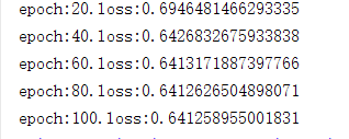

 

logistic 回归并不能很好的区分开这个复杂的数据集。使用神经网络
 代码：

import torch
import numpy as np
from torch import nn
from torch.autograd import Variable
import torch.nn.functional as F
import matplotlib.pyplot as plt

def plot_decision_boundary(model,x,y):
    #Set min and max values and give it some padding
    x_min,x_max=x[:,0].min()-1,x[:,0].max()+1
    y_min,y_max=x[:,1].min()-1,x[:,1].max()+1
    h=0.01
    #Generate a grid of points with distance h between them
    xx,yy=np.meshgrid(np.arange(x_min,x_max,h),np.arange(y_min,y_max,h))
    #Predict the function value for the whole grid
    Z=model(np.c_[xx.ravel(),yy.ravel()])
    Z=Z.reshape(xx.shape)
    #plot the contour and training examples
    plt.contourf(xx,yy,Z,cmap=plt.cm.Spectral)
    plt.ylabel('x2')
    plt.xlabel('x1')
    plt.scatter(x[:,0],x[:,1],c=y.reshape(-1),s=40,cmap=plt.cm.Spectral)
    plt.show()

np.random.seed(1)
m=400#样本数量
N=int(m/2)#每一类点的个数
D=2#维度
x=np.zeros((m,D))
y=np.zeros((m,1),dtype='uint8')#label 向量，0表示红色，1表示蓝色
a=4

for j in range(2):
    ix=range(N*j,N*(j+1))
    t=np.linspace(j*3.12,(j+1)*3.12,N)+np.random.rand(N)*0.2
    r=a*np.sin(4*t)+np.random.rand(N)*0.2
    x[ix]=np.c_[r*np.sin(t),r*np.cos(t)]
    y[ix]=j

plt.scatter(x[:,0],x[:,-1],c=y.reshape(-1),s=40,cmap=plt.cm.Spectral)
plt.show()

#首先使用logistic回归解决
x=torch.from_numpy(x).float()
y=torch.from_numpy(y).float()

w=nn.Parameter(torch.randn(2,1))
b=nn.Parameter(torch.zeros(1))

optimizer=torch.optim.SGD([w,b],1e-1)

def logistic_regression(x):
    return torch.mm(x,w)+b

criterion=nn.BCEWithLogitsLoss()

for e in range(100):
    out=logistic_regression(Variable(x))
    loss=criterion(out,Variable(y))
    optimizer.zero_grad()
    loss.backward()
    optimizer.step()
    if(e+1)%20==0:
        print('epoch:{}.loss:{}'.format(e+1,loss.item()))

def plot_logistic(x):
    x=Variable(torch.from_numpy(x).float())
    out=F.sigmoid(logistic_regression(x))
    out=(out>0.5)*1
    return out.data.numpy()

plot_decision_boundary(lambda x:plot_logistic(x),x.numpy(),y.numpy())
plt.title('logistic regression')

#定义两层神经网络的参数
w1=nn.Parameter(torch.randn(2,4)*0.01)#隐藏层神经元个数2
b1=nn.Parameter(torch.zeros(4))

w2=nn.Parameter(torch.randn(4,1)*0.01)
b2=nn.Parameter(torch.zeros(1))

#定义模型
def two_network(x):
    x1=torch.mm(x,w1)+b1
    x1=F.tanh(x1)#使用的PyTorch自带的tanh激活函数
    x2=torch.mm(x1,w2)+b2
    return x2

optimizer=torch.optim.SGD([w1,w2,b1,b2],1.)
criterion=nn.BCEWithLogitsLoss()
#训练10000次
for e in range(10000):
    out=two_network(Variable(x))
    loss=criterion(out,Variable(y))
    optimizer.zero_grad()
    loss.backward()
    optimizer.step()
    if(e+1)%10000==0:
        print('epoch:{},loss:{}'.format(e+1,loss.item()))

def plot_network(x):
    x=Variable(torch.from_numpy(x).float())
    x1=torch.mm(x,w1)+b1
    x1=F.tanh(x1)
    x2=torch.mm(x1,w2)+b2
    out=F.sigmoid(x2)
    out=(out>0.5)*1
    return out.data.numpy()

plot_decision_boundary(lambda x:plot_network(x),x.numpy(),y.numpy())
plt.title('2 layer network')

 可以看到神经网络能够非常好地分类这个复杂的数据，和前面的logistic回归相比，神经网络因为有了激活函数的存在，成了一个非线性分类器，所以神经网络分类的边界更加复杂。

Sequential和Module

使用Sequential和Module定义上面的神经网络：

#Sequential
seq_net=nn.Sequential(
    nn.Linear(2,4),#pyTorch中的线性层，wx+b
    nn.Tanh(),
    nn.Linear(4,1)
)
#序列模块可以通过索引访问每一层
seq_net[0]#第一层
print(seq_net[0])
#打印出第一层的权重
w0=seq_net[0].weight
print(w0)

 PyTorch自带的模块比自己写的更加稳定。

import torch
import numpy as np
from torch import nn
from torch.autograd import Variable
import torch.nn.functional as F
import matplotlib.pyplot as plt

def plot_decision_boundary(model,x,y):
    #Set min and max values and give it some padding
    x_min,x_max=x[:,0].min()-1,x[:,0].max()+1
    y_min,y_max=x[:,1].min()-1,x[:,1].max()+1
    h=0.01
    #Generate a grid of points with distance h between them
    xx,yy=np.meshgrid(np.arange(x_min,x_max,h),np.arange(y_min,y_max,h))
    #Predict the function value for the whole grid
    Z=model(np.c_[xx.ravel(),yy.ravel()])
    Z=Z.reshape(xx.shape)
    #plot the contour and training examples
    plt.contourf(xx,yy,Z,cmap=plt.cm.Spectral)
    plt.ylabel('x2')
    plt.xlabel('x1')
    plt.scatter(x[:,0],x[:,1],c=y.reshape(-1),s=40,cmap=plt.cm.Spectral)
    plt.show()

np.random.seed(1)
m=400#样本数量
N=int(m/2)#每一类点的个数
D=2#维度
x=np.zeros((m,D))
y=np.zeros((m,1),dtype='uint8')#label 向量，0表示红色，1表示蓝色
a=4

for j in range(2):
    ix=range(N*j,N*(j+1))
    t=np.linspace(j*3.12,(j+1)*3.12,N)+np.random.rand(N)*0.2
    r=a*np.sin(4*t)+np.random.rand(N)*0.2
    x[ix]=np.c_[r*np.sin(t),r*np.cos(t)]
    y[ix]=j

plt.scatter(x[:,0],x[:,-1],c=y.reshape(-1),s=40,cmap=plt.cm.Spectral)
plt.show()

#首先使用logistic回归解决
x=torch.from_numpy(x).float()
y=torch.from_numpy(y).float()

w=nn.Parameter(torch.randn(2,1))
b=nn.Parameter(torch.zeros(1))

optimizer=torch.optim.SGD([w,b],1e-1)

def logistic_regression(x):
    return torch.mm(x,w)+b

criterion=nn.BCEWithLogitsLoss()


def plot_logistic(x):
    x=Variable(torch.from_numpy(x).float())
    out=F.sigmoid(logistic_regression(x))
    out=(out>0.5)*1
    return out.data.numpy()

plot_decision_boundary(lambda x:plot_logistic(x),x.numpy(),y.numpy())
plt.title('logistic regression')



#Sequential
seq_net=nn.Sequential(
    nn.Linear(2,4),#pyTorch中的线性层，wx+b
    nn.Tanh(),
    nn.Linear(4,1)
)

#通过parameters可以取得模型的参数
param=seq_net.parameters()

#定义优化器
optim=torch.optim.SGD(param,1.)
#训练10000次
for e in range(10000):
    out=seq_net(Variable(x))
    loss=criterion(out,Variable(y))
    optim.zero_grad()
    loss.backward()
    optim.step()
    if(e+1)%1000==0:
        print('epoch:{},loss:{}'.format(e+1,loss.item()))

def plot_seq(x):
    out=F.sigmoid(seq_net(Variable(torch.from_numpy(x).float()))).data.numpy()
    out=(out>0.5)*1
    return out

plot_decision_boundary(lambda x:plot_seq(x),x.numpy(),y.numpy())
plt.title('sequential')

 

 保存模型：

#将参数和模型保存在一起(第一个参数是要保存的模型，第二个参数是保存的路径)

torch.save(seq_net,'save_seq_net.pth')

#读取保存的模型

seq_net1=torch.load('save_seq_net.pth') 

# 只保存模型参数，而不保存模型

torch.save(seq_net.state_dict(),'save_net_params.'pth)

#重新读入参数

seq_net2=nn.Sequential(

    nn.Linear(2,4),

    nn.Tanh(),

    nn.Linear(4,1)

) 

seq_net2.load_state_dict(torch.load('save_seq_net_params.pth'))

Module模板：

class 网络名字(nn.Module):
    def __init__(self,一些定义的参数):
        super(网路名,self).__init__()
        self.layer1=nn.Linear(num_input,num_hidden)
        self.layer2=nnn.Sequential(……)
        ……
        定义需要用的网络层
        
    def forward(self,x):#定义前向传播
        x1=self.layer1(x)
        x2=self.layer2(x)
        x=x1+x2
        ……
        return x
    

按照模板实现上面的神经网络：

import torch
import numpy as np
from torch import nn
from torch.autograd import Variable
import torch.nn.functional as F
import matplotlib.pyplot as plt

def plot_decision_boundary(model,x,y):
    #Set min and max values and give it some padding
    x_min,x_max=x[:,0].min()-1,x[:,0].max()+1
    y_min,y_max=x[:,1].min()-1,x[:,1].max()+1
    h=0.01
    #Generate a grid of points with distance h between them
    xx,yy=np.meshgrid(np.arange(x_min,x_max,h),np.arange(y_min,y_max,h))
    #Predict the function value for the whole grid
    Z=model(np.c_[xx.ravel(),yy.ravel()])
    Z=Z.reshape(xx.shape)
    #plot the contour and training examples
    plt.contourf(xx,yy,Z,cmap=plt.cm.Spectral)
    plt.ylabel('x2')
    plt.xlabel('x1')
    plt.scatter(x[:,0],x[:,1],c=y.reshape(-1),s=40,cmap=plt.cm.Spectral)
    plt.show()

np.random.seed(1)
m=400#样本数量
N=int(m/2)#每一类点的个数
D=2#维度
x=np.zeros((m,D))
y=np.zeros((m,1),dtype='uint8')#label 向量，0表示红色，1表示蓝色
a=4


for j in range(2):
    ix=range(N*j,N*(j+1))
    t=np.linspace(j*3.12,(j+1)*3.12,N)+np.random.rand(N)*0.2
    r=a*np.sin(4*t)+np.random.rand(N)*0.2
    x[ix]=np.c_[r*np.sin(t),r*np.cos(t)]
    y[ix]=j

x=torch.from_numpy(x).float()
y=torch.from_numpy(y).float()

class module_net(nn.Module):
    def __init__(self,num_input,num_hidden,num_output):
        super(module_net,self).__init__()
        self.layer1=nn.Linear(num_input,num_hidden)
        self.layer2=nn.Tanh()
        self.layer3=nn.Linear(num_hidden,num_output)

    def forward(self,x):#定义前向传播
        x=self.layer1(x)
        x=self.layer2(x)
        x=self.layer3(x)
        return x

mo_net=module_net(2,4,1)

#访问模型中的某次可以直接通过名字
#第一层
l1=mo_net.layer1
print(l1)
#打印出第一层的权重
print(l1.weight)

criterion=nn.BCEWithLogitsLoss()

#定义优化器
optim=torch.optim.SGD(mo_net.parameters(),1)

#训练10000次
for e in range(10000):
    out=mo_net(Variable(x))
    loss=criterion(out,Variable(y))
    optim.zero_grad()
    loss.backward()
    optim.step()
    if(e+1)%1000==0:
        print('epoch:{},loss:{}'.format(e+1,loss.item()))


#保存模型
torch.save(mo_net.state_dict(),'module_net.pth')