梯度下降法-单变量线性回归

1. load(‘data1.txt’)

将 data1.txt 放在桌面，更改MATLAB的当前文件夹到桌面，如下图（即在当前文件夹中包含 data1.txt）：
在这里插入图片描述
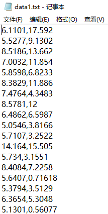
数据集样例如下图：

第一列为 x，第二列为 y，导入数据集，代码如下：

data = load('data1.txt');
x = data(:,1); % x 为data第一列
y = data(:,2); % y 为data第二列

2. 定义参数

首先定义单变量线性回归（即确定直线y=w0+w1*x）的参数 w0 和 w1，写成列向量形式，并初始化：

W = [0, 0];  % 初始化 w0=0，w1=0

再分别定义学习率 alpha 和阈值 total_loss：

当相邻两次迭代的损失函数loss（W）的差小于阈值时，则认为损失函数loss(W)收敛，也即循环终止条件：

alpha = 0.002;    % 学习率
total_loss = 0.00001;    % 阈值

3. 初始化

grad = [0, 0];
grad(1) = mean(w(1) + w(2) .* x - y);
grad(2) = mean(x .* (w(1) + w(2) .* x - y));
loss = (mean((w(1) + w(2) * x - y) .^ 2));
w = w - alpha .* grad;
loss_new = (mean((w(1) + w(2) * x - y) .^ 2));

代码解释如下：
在这里插入图片描述

4. 迭代

while 1
    w = w - alpha .* grad;
    grad(1) = mean(w(1) + w(2) .* x - y);
    grad(2) = mean(x .* (w(1) + w(2) .* x - y));
    loss = loss_new;
    loss_new = (mean((w(1) + w(2) .* x - y) .^ 2));
    if abs(loss_new - loss) < total_loss
        f = w(2) .* x + w(1);
        plot(x,y,'r+',x,f);
        break;
    end
end

按照更新规则更新 w，grad，loss 和 loss_new，直到 abs(loss_new - loss) （即连续两次迭代损失函数的差值的平方）小于之前定义的阈值total_loss，则循环终止，得到参数 w0 和w1。
f = w(2) .* x + w(1) 即线性回归需要确定的直线；
plot(x,y,‘r+’,x,f)即分别把 data1.txt中的点和拟合的直线f画出来。

5. 完整代码

data = load('data1.txt');
x = data(:,1);
y = data(:,2);

w = [0, 0];  % 参数
alpha = 0.002;    % 学习率
total_loss = 0.00001;    % 阈值

% 初始化
grad = [0, 0];
grad(1) = mean(w(1) + w(2) .* x - y);
grad(2) = mean(x .* (w(1) + w(2) .* x - y));
loss = (mean((w(1) + w(2) * x - y) .^ 2));
w = w - alpha .* grad;
loss_new = (mean((w(1) + w(2) * x - y) .^ 2));

% 迭代
while 1
    w = w - alpha .* grad;
    grad(1) = mean(w(1) + w(2) .* x - y);
    grad(2) = mean(x .* (w(1) + w(2) .* x - y));
    loss = loss_new;
    loss_new = (mean((w(1) + w(2) .* x - y) .^ 2));
    if abs(loss_new - loss) < total_loss
        f = w(2) .* x + w(1);
        plot(x,y,'r.',x,f);
        break;
    end
end

注意 alpha 和total_loss 的值自行设置
注意 plot(x,y,‘r.’,x,f)中的‘r.’代表用“.”描点，作图结果如下：

6.另附课堂代码（最小二乘法）

在这里插入图片描述

data=load('data1.txt'); 
A=[ones(size(data,1),1),data(:,1)];
a=data(:,1);
b=data(:,2);
w=A\b;
w0=w(1,:);
w1=w(2,:);
Y=w1*a+w0;
plot(a,b, 'r*', 'MarkerSize', 10);
hold on;
plot(a,Y);

运行结果如图：
在这里插入图片描述

7.data2.txt代码

data = load('data2.txt');
positive = data(1:45,:);
negative = data(46:100,:);
scatter(positive(:,1),positive(:,2),'ro');
hold on;
scatter(negative(:,1),negative(:,2),'go');

x = positive';
y = negative';
d = 2;

for i=1:45
   A(i,:) = [-x(:,i)',-1];
end
for i=1:55
   A(i+45,:) = [y(:,i)',1];
end
c = ones(100,1)*(-1);
w = linprog(zeros(d+1,1),A,c);
hold on;
x1 = 3:8;
y1 = (-w(3)-w(1)*x1)/w(2);
plot(x1,y1,'-','LineWidth',2);

基于梯度下降法的单变量线性回归（MATLAB）