【动手学——Linear Regression】day01_Linear Regression两种方法实现

线性回归

一、基本组成元素

模型、数据集、损失函数、优化函数-随机梯度下降

二、代码讲解

代码完整版本地址url:

https://www.kesci.com/org/boyuai/project/5e4117b1b8c462002d687509

①从零开始实现

# import packages and modules
%matplotlib inline
import torch
from IPython import display
from matplotlib import pyplot as plt
import numpy as np
import random

print(torch.__version__)

下面开始操作

1.生成数据集

使用线性模型来生成数据集，生成一个1000个样本的数据集，下面是用来生成数据的线性关系：

traning data set、 sample、 feature、 lable:
我们通常收集一系列的真实数据，例如多栋房屋的真实售出价格和它们对应的面积和房龄。我们希望在这个数据上面寻找模型参数来使模型的预测价格与真实价格的误差最小。在机器学习术语里，该数据集被称为训练数据集（training data set）或训练集（training set），一栋房屋被称为一个样本（sample），其真实售出价格叫作标签（label），用来预测标签的两个因素叫作特征（feature）。特征用来表征样本的特点。

代码：

#特征数量
num_inputs = 2
#样本数量
num_examples = 1000

#设置真实的权重和偏差
#在这里设置这两个参数是因为，需要通过特征生成对应的标签
true_w = [2, -3.4]
true_b = 4.2

#下面这句生成特征
features = torch.randn(num_examples, num_inputs,
                      dtype=torch.float32)
                      
#通过特征生成标签，
labels = true_w[0] * features[:, 0] + true_w[1] * features[:, 1] + true_b

#现实中的数据不可能完全遵守线性模型，
#所以在末尾加上一个随机生成的偏
labels += torch.tensor(np.random.normal(0, 0.01, size=labels.size()),
                       dtype=torch.float32)

---

2.使用图像来展示生成的数据

#用向量图svg的形式展示数据集
def use_svg_display():
	display.set_matplotlib_formats('svg')
#设置展示图的大小
def set_figsize(figsize=(3.5,2.5)):
	use_svg_display()
	plt.rcParams['figure.figsize']=figsize
	
#先调用set_figsize设置大小
#再调用scatter函数打印展示数据集
set_figsize()
plt.scatter(features[:, 1].numpy(), labels.numpy(), 1);

3.读取数据集

def data_iter(batch_size, features, labels):
    num_examples = len(features)
    indices = list(range(num_examples))
   #用random.shuffle来打乱数据集的顺序
    random.shuffle(indices) 
    #取i到i+batch_size作为训练数据集，但是i+batch_size可能会超过数据集的上限1000，所以用min取小的那个
    for i in range(0, num_examples, batch_size):
        j = torch.LongTensor(indices[i: min(i + batch_size, num_examples)])
        yield  features.index_select(0, j), labels.index_select(0, j)

#设置数据集长度为10，取一批瞧瞧看
batch_size = 10

for X, y in data_iter(batch_size, features, labels):
    print(X, '\n', y)
    break

4.初始化模型参数

w = torch.tensor(np.random.normal(0, 0.01, (num_inputs, 1)), dtype=torch.float32)
b = torch.zeros(1, dtype=torch.float32)
#后面的优化函数会通过链式法则反向传播使用到参数的梯度
#所以需要在这里给模型的参数附上梯度
w.requires_grad_(requires_grad=True)
b.requires_grad_(requires_grad=True)

5.定义模型

#X:特征;需要训练的两个参数:权重w，偏差b
#特征与权重相加加上偏差即为预测值（y_hat）
def linreg(X, w, b):
    return torch.mm(X, w) + b

6.定义损失函数Loss Function

def squared_loss(y_hat, y): 
    return (y_hat - y.view(y_hat.size())) ** 2 / 2

7.定义优化函数

学习率: η 代表在每次优化中，能够学习的步长的大小
批量大小: B 是小批量计算中的批量大小batch size

总结一下，优化函数的有以下两个步骤：
(i)初始化模型参数，一般来说使用随机初始化；
(ii)我们在数据上迭代多次，通过在负梯度方向移动参数来更新每个参数。

def sgd(params, lr, batch_size): 
    for param in params:
        param.data -= lr * param.grad / batch_size 
        #使用.data避免对参数进行优化的动作累加

8.训练

当数据集、模型、损失函数和优化函数定义完了之后就可来准备进行模型的训练了。

# super parameters init/超参数设置
lr = 0.03		#学习率
num_epochs = 5	#训练周期（迭代次数）
#单层线性模型，均方误差函数
net = linreg	
loss = squared_loss

# training
#两个for循环
#大循环迭代整个过程，小循环取每一个sample出来计算并优化
for epoch in range(num_epochs):  
	# training repeats num_epochs times
    # in each epoch, all the samples in dataset will be used once/共迭代五次，每次都要把所有数据拿出来使用一次（batch_size）
    
    # X is the feature and y is the label of a batch sample
    for X, y in data_iter(batch_size, features, labels):
    	#将特征X、权重w、偏差b传入网络进行训练，得到对标签的预测值y_hat，再通过y、y_hat传入loss损失函数计算损失loss，并将其相加得到l
        l = loss(net(X, w, b), y).sum()  
        # towards backward to calculate the gradient of batch sample loss 
        l.backward()  
        # using small batch random gradient descent to iter model parameters
        #[w,b]:需要优化的参数；lr:学习率；batch_size：批量大小 
        sgd([w, b], lr, batch_size)  
        # reset parameter gradient/参数w,b梯度清零，避免梯度累加，影响下一次的计算结果
        w.grad.data.zero_()
        b.grad.data.zero_()
    train_l = loss(net(features, w, b), labels)
    print('epoch %d, loss %f' % (epoch + 1, train_l.mean().item()))

最后看一下训练结果的w、b与true_w、true_b的差距如何
差距越小代表我们的训练效果越好

---

② 基于pytorch的实现

#import some packages
import torch
from torch import nn
import numpy as np
torch.manual_seed(1)

print(torch.__version__)
torch.set_default_tensor_type('torch.FloatTensor')

1.生成数据集的操作和之前完全一样

2.读取数据集

import torch.utils.data as Data

batch_size = 10

# 将特征和标签组合起来组成数据集
dataset = Data.TensorDataset(features, labels)

# 使用Dataloader从数据集中取数据
data_iter = Data.DataLoader(
    dataset=dataset,            # torch TensorDataset format
    batch_size=batch_size,      # mini batch size
    shuffle=True,               # whether shuffle the data or not/是否随机取数据
    num_workers=2,              # 使用两个读数据线程来读数据
)

3.定义模型

class LinearNet(nn.Module):
	#网络参数的初始化
    def __init__(self, n_feature):
        super(LinearNet, self).__init__()      # call father function to init 
        self.linear = nn.Linear(n_feature, 1)  # function prototype: `torch.nn.Linear(in_features, out_features, bias=True)`
	#forward定义了数据在线性网络中如何传播
    def forward(self, x):
        y = self.linear(x)
        return y
#前面是类的定义，这里是实例化网络    
net = LinearNet(num_inputs)
print(net)

下面是生成多层网络的三种方法

# ways to init a multilayer network
# method one
net = nn.Sequential(
    nn.Linear(num_inputs, 1)
    # other layers can be added here
    )

# method two：调用add_module函数
net = nn.Sequential()
net.add_module('linear', nn.Linear(num_inputs, 1))
# net.add_module ......

# method three：与第一种类似，将网络加入到一个有序字典中
from collections import OrderedDict
net = nn.Sequential(OrderedDict([
          ('linear', nn.Linear(num_inputs, 1))
          # ......
        ]))

print(net)
print(net[0])

将整个网络和第一层打印出来看看：

两者是一样的，因为我们只生成了一层线性网络

4.初始化模型参数

模型构建完成后，用init这个模块进行模型参数的初始化

from torch.nn import init

init.normal_(net[0].weight, mean=0.0, std=0.01)
init.constant_(net[0].bias, val=0.0)  # or you can use `net[0].bias.data.fill_(0)` to modify it directly

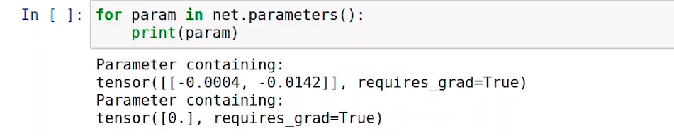
for param in net.parameters():
    print(param)

看一下初始化的模型参数
已经是自动附加了梯度的，无需手动添加

5.定义损失函数

loss = nn.MSELoss()    # nn built-in squared loss function
                       # function prototype: `torch.nn.MSELoss(size_average=None, reduce=None, reduction='mean')`

6.定义优化函数

优化函数选用随机梯度下降，是optim模块定义好的，直接调用

import torch.optim as optim
#随机梯度下降函数SGD的两个参数
#一个是我们要优化的参数w、b，一个是超参数学习率lr
optimizer = optim.SGD(net.parameters(), lr=0.03)   # built-in random gradient descent function
print(optimizer)  # function prototype: `torch.optim.SGD(params, lr=, momentum=0, dampening=0, weight_decay=0, nesterov=False)`

see see优化函数长啥样：

7.训练

num_epochs = 3
for epoch in range(1, num_epochs + 1):
    for X, y in data_iter:
        output = net(X)					# output即为y_hat
        l = loss(output, y.view(-1, 1))	# y与y_hat求出损失
        optimizer.zero_grad() 			# reset gradient, equal to net.zero_grad()/梯度清零，避免对下一次计算产生累加影响
        l.backward()
        optimizer.step()				# 通过optimzer对象使用优化函数进行优化
    print('epoch %d, loss: %f' % (epoch, l.item()))

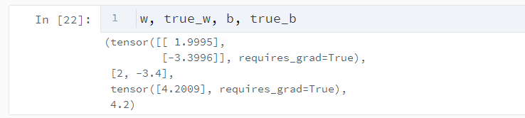
看一下如何最后训练的参数和实际的参数的差距：

# result comparision
dense = net[0]
print(true_w, dense.weight.data)
print(true_b, dense.bias.data)

非常接近，说明训练的效果不错

---

两种实现方式的比较
从零开始的实现（推荐用来学习）
能够更好的理解模型和神经网络底层的原理

使用pytorch的简洁实现
能够更加快速地完成模型的设计与实现

---

习题及解释：

1.

解答：
有几个输出节点，b的个数就是几
题中输入是78,输出是71，7是批量大小（batch_size），所以输入节点有8个，输出节点是1个。所以b的个数也是1

2.

y_hat的形状是[n, 1]，而y的形状是[n]，两者相减得到的结果的形状是[n, n]，相当于用y_hat的每一个元素分别减去y的所有元素，所以无法得到正确的损失值。对于第一个选项，y_hat.view(-1)的形状是[n]，与y一致，可以相减；对于第二个选项，y.view(-1)的形状仍是[n]，所以没有解决问题；对于第三个选项和第四个选项，y.view(y_hat.shape)和y.view(-1, 1)的形状都是[n, 1]，与y_hat一致，可以相减。
以下是一段示例代码：
x = torch.arange(3)
y = torch.arange(3).view(3, 1)
print(x)
print(y)
print(x + y)
[10]、[10,1]形状区别
view()用法
改变形状