小白_从0开始学习_FashionMNIST_深度学习_卷积神经网络_pytorch代码详解

FashionMNIST_深度学习_pytorch代码详解

关于其中不解的地方，如输出，输入节点的数值不知怎么计算。或是哪块代码不清楚。又或是想要我在手中测试的完整代码请在下方留下您的QQ或邮箱

from resources.plot_confusion_matrix import plot_confusion_matrix

文中该函数是我自己写的，如果有需要也请在评论区留下你的QQ或邮箱

概要

FashionMNIST 是一个替代 MNIST 手写数字集 的图像数据集。 可以说是MNIST的升级版，它来自 10 种类别的共 7 万个不同商品的图片。
FashionMNIST 的大小、格式和训练集/测试集划分与原始的 MNIST 完全一致。60000/10000 的训练测试数据划分，28x28 的灰度图片。
进行FashionMNIST数据深度学习测试时，首先要安装pytorch这个库，也可以用其它的库，像是TensorFlow之类的。

整体流程概述

一 准备过程
1.引入各种包和库
2.数据的加载
.3.数据的处理
4.网络的搭建
二 The Training Process(训练过程)
1.Get batch from training set(从训练集中获取批次)
2.Pass batch to network(将此批次送入网络中)
3.Calculate the loss(计算损失)
4.Calculate the gradient(计算损失梯度)
5.Updat the weights using the gradient to reduce the loss(渐变权重梯度减小损失)
6.repeat steps1-5 until one epoch is completed(重复步骤1-5直到一个epoch完成)
7.repeat step 1-6

代码开始

准备过程

1.import库

import torch
import torch.nn as nn
import torch.nn.functional as F

import torch.optim as optim  #优化器 to uodate weights

import torchvision
import torchvision.transforms as transforms

torch.set_printoptions(linewidth=120)#设置输出格式
torch.set_grad_enabled(True)

2. 数据加载

改代码从网络上下载FashionMNIST数据集
并保存到c:/code（自定义）中

train_set=torchvision.datasets.FashionMNIST(
    root='c:/code'
    ,train=True
    ,download=True
    ,transform=transforms.Compose([   #调整数据格式为tensor
        transforms.ToTensor()   
    ])
)

把数据分批 100份数据为一批

train_loader=torch.utils.data.DataLoader(train_set,batch_size=100)
batch=next(iter(train_loader))
images,labels=batch

3.网络建立

class Network(nn.Module):
    def __init__(self):
        super(Network,self).__init__()
        #self.layer = None
        self.conv1=nn.Conv2d(in_channels=1,out_channels=6,kernel_size=5)#in_channels 处理灰度图像 gray=1
        self.conv2=nn.Conv2d(in_channels=6,out_channels=12,kernel_size=5)
        """
        kernel_size 设置过滤器大小 卷积滤波器
        out_channels 设置过滤器数量，输出渠道，输出一级张量
        out_features 
        """
         
        self.fc1=nn.Linear(in_features=12*4*4,out_features=120)
        self.fc2=nn.Linear(in_features=120,out_features=60)
        self.out=nn.Linear(in_features=60,out_features=10)#out_features 取决于类的数量 num_labels
    def forward(self,t):
        #t = self.layer(t)
        #(1) input layer
        t=t
        
        #(2) hidden conv layer
        t=self.conv1(t)
        t=F.relu(t)
        t=F.max_pool2d(t,kernel_size=2,stride=2)
        
        #(3) hidden conv layer
        t=self.conv2(t)
        t=F.relu(t)
        t=F.max_pool2d(t,kernel_size=2,stride=2)
        
        #hidden liner layer
        t=t.reshape(-1,12*4*4)
        t=self.fc1(t)
        t=F.relu(t)
        
        #hidden liner layer
        t=self.fc2(t)
        t=F.relu(t)                         #用relu作为激活功能
        
        #output layer
        t=self.out(t)
        #t=F.softmax(t,dim=1)       #预测概率最大值  loss function
        return t

写一个计算准确率的函数

def get_num_correct(preds,labels):
    return preds.argmax(dim=1).eq(labels).sum().item()

训练过程

1.Get batch from training set(从训练集中获取批次)

network=Network()
train_loader=torch.utils.data.DataLoader(train_set,batch_size=100)
optimizer=optim.Adam(network.parameters(),lr=0.01)#SGD lr 学习率    第一个为网络参数

2.Pass batch to network(将此批次送入网络中)

		batch=next(iter(train_loader))
		images,labels=batch
        preds=network(images)#pass batch

3.Calculate the loss(计算损失)

loss=F.cross_entropy(preds,labels)#Calculate Loss

4.Calculate the gradient(计算损失梯度)

loss.backward()#Calculate Gradients

5.Updat the weights using the gradient to reduce the loss(渐变权重梯度减小损失)

// An highlighted block
optimizer.step()#updata weights

6.repeat steps1-5 until one epoch is completed(重复步骤1-5直到一个epoch完成)

第六步其实就是把step1-5整合起来写一个for循环

7.repeat step 1-6

在第六步的for外面在来一层for

备注

在第六步中的for循环中每计算完损失后，要把梯度置0
用以下代码

optimizer.zero_grad()

开始进行预测Predicitions

建立获取预测并保存测试集结果的函数

def get_all_preds(model,loader):
    all_preds=torch.tensor([])
    for batch in loader:
        images,labels=batch
        
        preds=model(images)
        all_preds=torch.cat(
            (all_preds,preds),
            dim=0
        )
    return all_preds

测试集数据加载

pre_loader=torch.utils.data.DataLoader(train_set,batch_size=10000)
train_preds=get_all_preds(network,pre_loader)

准确率获取

preds_correct=get_num_correct(train_preds,train_set.targets)
print('total correct:',preds_correct)

建立混淆矩阵

先把真实值和测试值两两对应放在一起

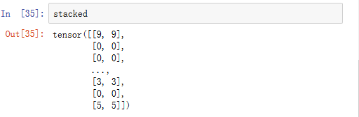
stacked = torch.stack(
    (
    train_set.targets
    ,train_preds.argmax(dim=1)
    ),dim=1
)

该代码运行结果如下：
建立一个10×10的空白矩阵cmt

cmt=torch.zeros(10,10,dtype=torch.int32)

之后进行统计预测的结果

for p in stacked:
    j,k=p.tolist()
    cmt[j,k]+=1

代码运行结果如下：

###之后画出混淆矩阵

import matplotlib.pyplot as plt
from sklearn.metrics import confusion_matrix
from resources.plot_confusion_matrix import plot_confusion_matrix
name=('T-shirt','Trouser','Pullover','Dress','Coat','Sandal','Shirt','Sneaker','Bag','Anke')
plt.figure(figsize=(10,10))
plot_confusion_matrix(cm,name)

代码结果如下：

章末

from resources.plot_confusion_matrix import plot_confusion_matrix

该函数是我自己写的，如果有需要请在评论区留下你的QQ或邮箱

鄙人拙作,有不当之处,还请指教