Python金融科技:cufflinks绘制金融图表

前言

最近发现一个功能强大的绘图工具库cufflinks，其最吸引我的地方是内置了量化金融绘图模块，可以很方便地绘制K线和技术指标图表。但遗憾的是，在网络上并没有找到cufflinks的参考手册。虽然网络上有一些介绍cufflinks的博客文章，但都没有详细介绍量化绘图模块的使用方法。

因此本蒟蒻参照cufflinks的github源码，对cufflinks量化金融绘图模块的使用方法做出简要的介绍，希望对您有些许帮助。

cufflinks介绍

cufflinks是对Python绘图库plotly的进一步封装，是基于jupyter notebook的交互式绘图工具，可以很方便地绘制各种交互式图表，布局优美，效果炫酷，操作方便，可以和pandas的数据类型无缝衔接。

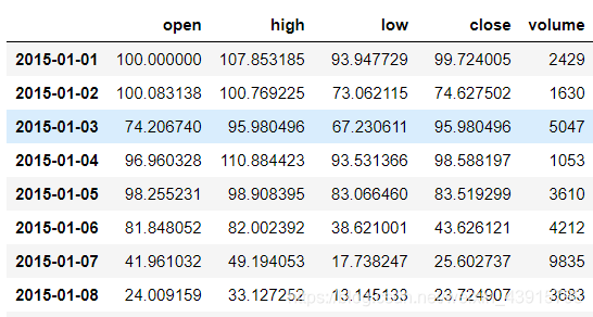
cufflinks的量化金融绘图模块接收的金融交易数据为，dataframe格式，index为datetime类型，各列为open、high、low、close、volume，如下：

使用方法

注意：目前cufflinks只能在jupyter notebook中使用，在其他的IDE中使用可能会无法 编译执行。

因为本蒟蒻水平有限，如有错误，欢迎批评指正。

笔者的环境：cufflinks 0.17.3、Python3.7 、Jupyter Notebook

更多信息可以参考cufflinks的源码

安装cufflinks：

pip install cufflinks

1.绘制基础K线（蜡烛）图

import cufflinks as cf
cf.set_config_file(offline=True, world_readable=True)
df=cf.datagen.ohlcv()#cufflinks提供的数据，也可以更改为自定义数据
qf=cf.QuantFig(df,title='cufflinks金融绘图样例',legend='top',name='QF')
qf.iplot()

效果图:

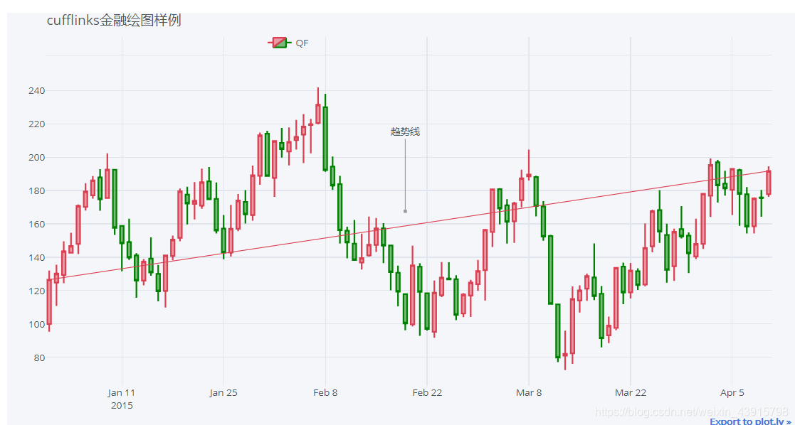
2.添加趋势线

import cufflinks as cf
cf.set_config_file(offline=True, world_readable=True)
qf=cf.QuantFig(df,title='cufflinks金融绘图样例',legend='top',name='QF')
qf.add_trendline('2015-01-01','2015-04-10',on='close',text='趋势线',textangle=0)#画趋势线，textangle设置文字角度
qf.iplot(up_color='red',down_color='green')

效果图：

参数介绍（摘自源码注释）：

"""
		Parameters:
			date0 : string
				Trendline starting date
			date1 :  string
				Trendline end date
			on : string
				Indicate the data series in which the 
				trendline should be based.
					'close'
					'high'
					'low'
					'open'
			text : string
				If passed, then an annotation will be added 
				to the trendline (at mid point)
		kwargs:
			from_strfmt : string
				Defines the date formating in which 
				date0 and date1 are stated. 
				default: '%d%b%y'					
			to_strfmt : string
				Defines the date formatting 
				to which it should be converted. 
				This should match the same format as the timeseries index. 
				default : '%Y-%m-%d'		
"""

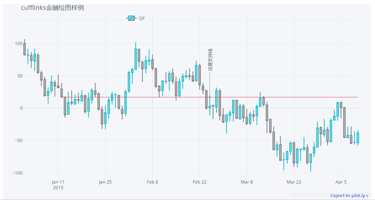
3.添加支撑线

import cufflinks as cf
cf.set_config_file(offline=True, world_readable=True)
qf=cf.QuantFig(df,title='cufflinks金融绘图样例',legend='top',name='QF')
qf.add_support('2015-01-12',on='close',mode='toend',text='这是支持线')
qf.iplot()

参数介绍：

"""
		Parameters:
			date0 : string
				The support line will be drawn at the 'y' level 
				value that corresponds to this date. 
			on : string
				Indicate the data series in which the 
				support line should be based.
					'close'
					'high'
					'low'
					'open'
			mode : string
				Defines how the support/resistance will 
				be drawn
					'starttoened' : (x0,x1)
					'fromstart' : (x0,date)
					'toend' : (date,x1)
			text : string
				If passed, then an annotation will be added 
				to the support line (at mid point)
		
		kwargs:	
			from_strfmt : string
				Defines the date formating in which 
				date0 and date1 are stated. 
				default: '%d%b%y'					
			to_strfmt : string
				Defines the date formatting 
				to which it should be converted. 
				This should match the same format as the timeseries index. 
				default : '%Y-%m-%d'		
		"""

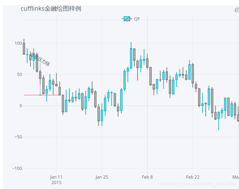
4.添加压力线

import cufflinks as cf
cf.set_config_file(offline=True, world_readable=True)
qf=cf.QuantFig(df,title='cufflinks金融绘图样例',legend='top',name='QF')
qf.add_resistance('2015-01-12',on='close',mode='fromstart',text='这是压力线',textangle=30)
qf.iplot()

效果图：
参数介绍：
与支撑线相似

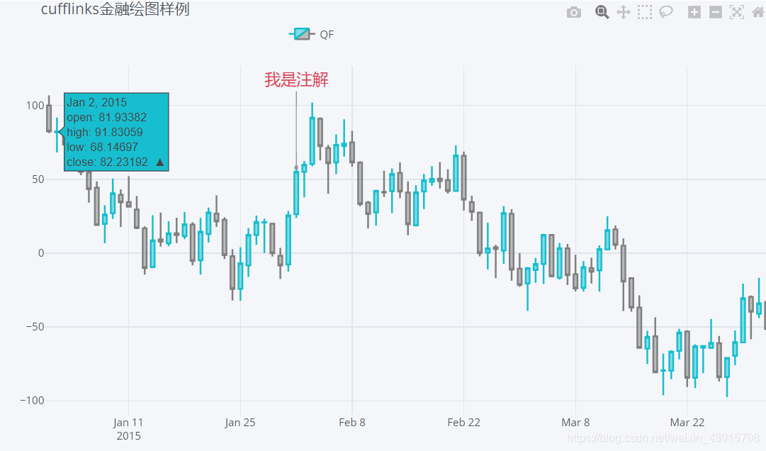
5.添加注解

import cufflinks as cf
cf.set_config_file(offline=True, world_readable=True)
qf=cf.QuantFig(df,title='cufflinks金融绘图样例',legend='top',name='QF')
qf.add_annotations({'2015-02-01':'我是注解'},fontcolor='red',fontsize=18,textangle=0)
qf.iplot()

效果图：

"""
		Parameters:
			annotations : dict or list(dict,)
				Annotations can be on the form form of 
					{'date' : 'text'}
					and the text will automatically be placed at the 
					right level on the chart 
				or
					A Plotly fully defined annotation
		kwargs : 
			fontcolor : str
				Text color for annotations
			fontsize : int
				Text size for annotations
			textangle : int
				Textt angle 
			See https://plot.ly/python/reference/#layout-annotations 
			for a complete list of valid parameters.
		"""

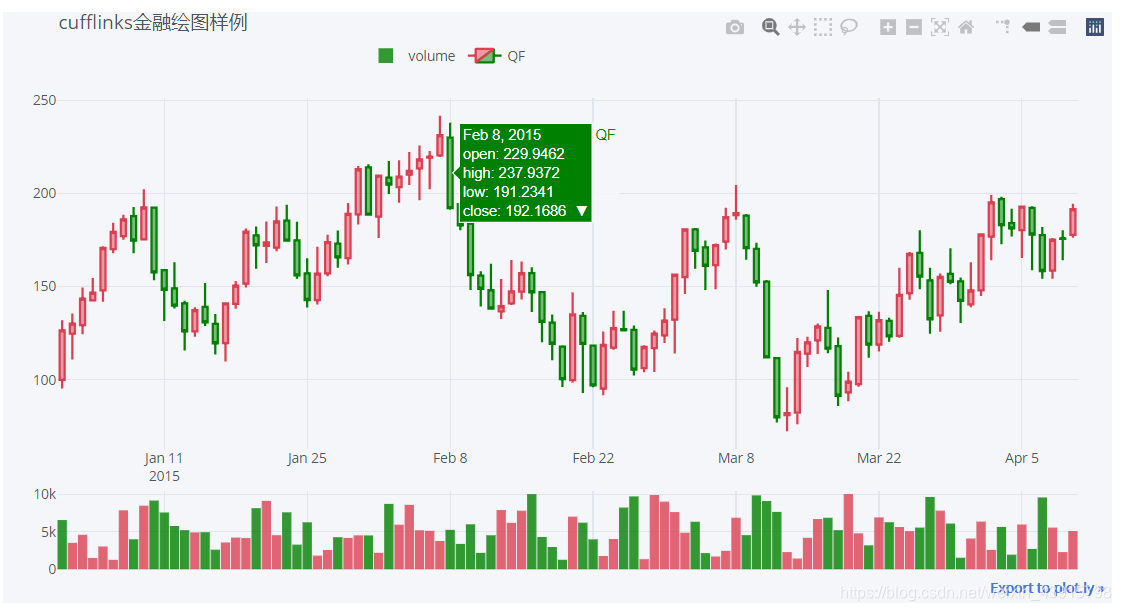
6.添加交易量

import cufflinks as cf
cf.set_config_file(offline=True, world_readable=True)
qf=cf.QuantFig(df,title='cufflinks金融绘图样例',legend='top',name='QF')
qf.add_volume()
qf.iplot(up_color='red',down_color='green')#可以设置主题颜色

效果图：

参数介绍：

"""
		Parameters:
			colorchange : bool
				If True then each volume bar will have a fill color 
				depending on if 'base' had a positive or negative
				change compared to the previous value
				If False then each volume bar will have a fill color 
				depending on if the volume data itself had a positive or negative
				change compared to the previous value
			column :string
				Defines the data column name that contains the volume data. 
				Default: 'volume'
			name : string
				Name given to the study
			str : string
				Label factory for studies
				The following wildcards can be used:
					{name} : Name of the column
					{study} : Name of the study
					{period} : Period used
				Examples:
					'study: {study} - period: {period}'
			
		kwargs : 
			base : string
				Defines the column which will define the
				positive/negative changes (if colorchange=True).
				Default = 'close'
			up_color : string
				Color for positive bars
			down_color : string
				Color for negative bars
		"""

7.添加异同移动平均线MACD

import cufflinks as cf
cf.set_config_file(offline=True, world_readable=True)
qf=cf.QuantFig(df,title='cufflinks金融绘图样例',legend='top',name='QF')
qf.add_macd()
qf.iplot()

效果图：

参数介绍：

"""
		Parameters:
			fast_period : int
				MACD Fast Period
			slow_period : int
				MACD Slow Period
			signal_period : int
				MACD Signal Period
			column :string
				Defines the data column name that contains the 
				data over which the study will be applied. 
				Default: 'close'
			name : string
				Name given to the study
			str : string
				Label factory for studies
				The following wildcards can be used:
					{name} : Name of the column
					{study} : Name of the study
					{period} : Period used
				Examples:
					'study: {study} - period: {period}'
		kwargs: 
			legendgroup : bool
				If true, all legend items are grouped into a 
				single one
			All formatting values available on iplot()
		"""

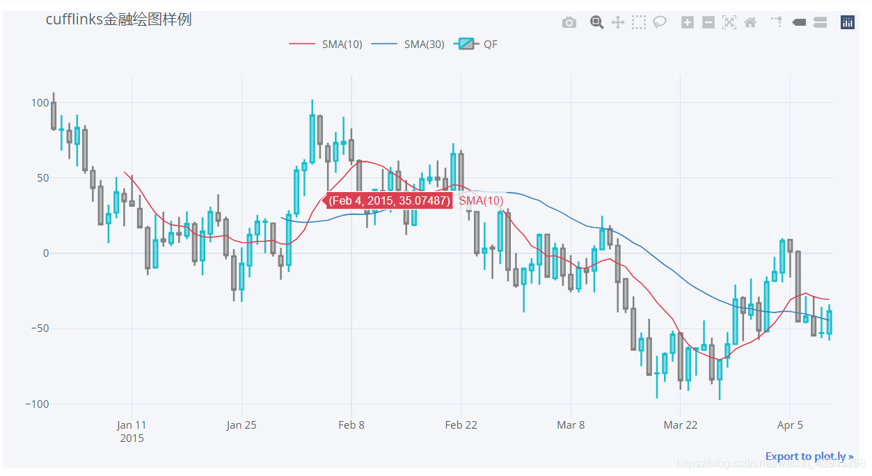
8.添加简单移动均线SMA

import cufflinks as cf
cf.set_config_file(offline=True, world_readable=True)
qf=cf.QuantFig(df,title='cufflinks金融绘图样例',legend='top',name='QF')
qf.add_sma(periods=[10,30],color=['red','blue'])
qf.iplot()

参数介绍：

"""
		Parameters:
			periods : int or list(int)
				Number of periods
			column :string
				Defines the data column name that contains the 
				data over which the study will be applied. 
				Default: 'close'
			name : string
				Name given to the study
			str : string
				Label factory for studies
				The following wildcards can be used:
					{name} : Name of the column
					{study} : Name of the study
					{period} : Period used
				Examples:
					'study: {study} - period: {period}'
		kwargs: 
			legendgroup : bool
				If true, all legend items are grouped into a 
				single one
			All formatting values available on iplot()
		"""

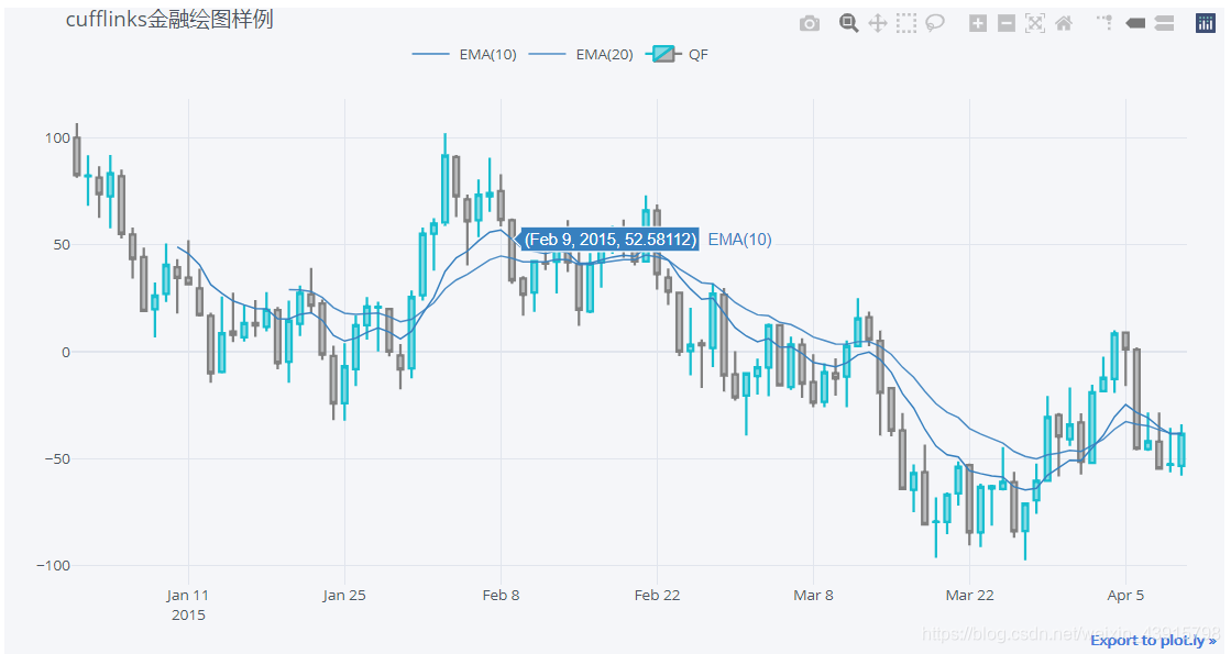
9.添加EMA

import cufflinks as cf
cf.set_config_file(offline=True, world_readable=True)
qf=cf.QuantFig(df,title='cufflinks金融绘图样例',legend='top',name='QF')
qf.add_ema(periods=[10,20])
qf.iplot()

效果图：

参数介绍：

"""
		Parameters:
			periods : int or list(int)
				Number of periods
			column :string
				Defines the data column name that contains the 
				data over which the study will be applied. 
				Default: 'close'
			name : string
				Name given to the study
			str : string
				Label factory for studies
				The following wildcards can be used:
					{name} : Name of the column
					{study} : Name of the study
					{period} : Period used
				Examples:
					'study: {study} - period: {period}'
		kwargs: 
			legendgroup : bool
				If true, all legend items are grouped into a 
				single one
			All formatting values available on iplot()
		"""

10.添加RSI

import cufflinks as cf
cf.set_config_file(offline=True, world_readable=True)
qf=cf.QuantFig(df,title='cufflinks金融绘图样例',legend='top',name='QF')
qf.add_rsi(periods=10)
qf.iplot()

效果图：

参数介绍：

"""
		Parameters:
			periods : int or list(int)
				Number of periods
			rsi_upper : int 
				bounds [0,100]
				Upper (overbought) level
			rsi_lower : int
				bounds [0,100]
				Lower (oversold) level
			showbands : boolean
				If True, then the rsi_upper and
				rsi_lower levels are displayed
			column :string
				Defines the data column name that contains the 
				data over which the study will be applied. 
				Default: 'close'
			name : string
				Name given to the study
			str : string
				Label factory for studies
				The following wildcards can be used:
					{name} : Name of the column
					{study} : Name of the study
					{period} : Period used
				Examples:
					'study: {study} - period: {period}'
		kwargs: 
			legendgroup : bool
				If true, all legend items are grouped into a 
				single one
			All formatting values available on iplot()
		"""

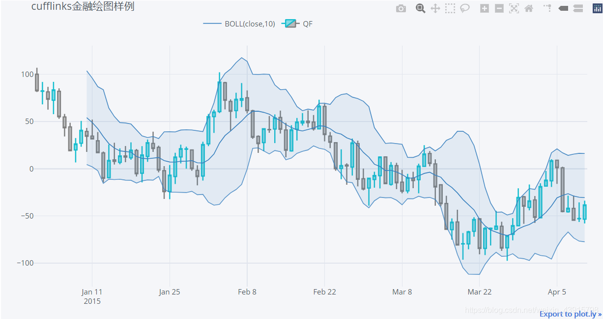
11.添加布林线

import cufflinks as cf
cf.set_config_file(offline=True, world_readable=True)
qf=cf.QuantFig(df,title='cufflinks金融绘图样例',legend='top',name='QF')
qf.add_bollinger_bands(periods=10)
qf.iplot()

效果图：

参数介绍：

"""
		Parameters:
			periods : int or list(int)
				Number of periods
			boll_std : int
				Number of standard deviations for
				the bollinger upper and lower bands
			fill : boolean
				If True, then the innner area of the 
				bands will filled
			column :string
				Defines the data column name that contains the 
				data over which the study will be applied. 
				Default: 'close'
			name : string
				Name given to the study
			str : string
				Label factory for studies
				The following wildcards can be used:
					{name} : Name of the column
					{study} : Name of the study
					{period} : Period used
				Examples:
					'study: {study} - period: {period}'
		kwargs: 
			legendgroup : bool
				If true, all legend items are grouped into a 
				single one
			fillcolor : string
				Color to be used for the fill color.
				Example:
					'rgba(62, 111, 176, .4)'
			All formatting values available on iplot()
		"""

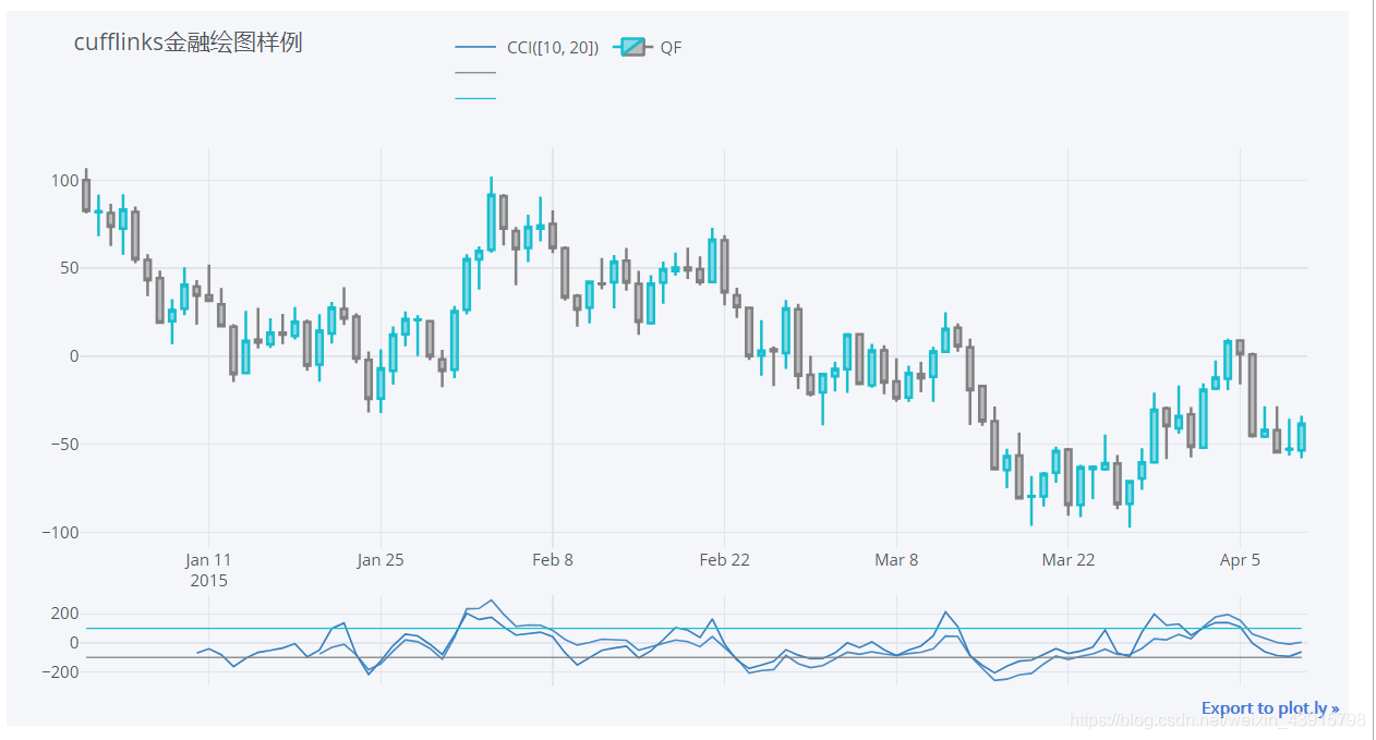
12.添加顺势指标/商品通道指标CCI

import cufflinks as cf
cf.set_config_file(offline=True, world_readable=True)
qf=cf.QuantFig(df,title='cufflinks金融绘图样例',legend='top',name='QF')
qf.add_cci(periods=[10,20])
qf.iplot()

效果图：

参数介绍：

"""
		Parameters:
			periods : int or list(int)
				Number of periods
			cci_upper : int
				Upper bands level
				default : 100
			cci_lower : int
				Lower band level
				default : -100
			showbands : boolean
				If True, then the cci_upper and
				cci_lower levels are displayed
			name : string
				Name given to the study
			str : string
				Label factory for studies
				The following wildcards can be used:
					{name} : Name of the column
					{study} : Name of the study
					{period} : Period used
				Examples:
					'study: {study} - period: {period}'
		kwargs: 
			legendgroup : bool
				If true, all legend items are grouped into a 
				single one
			All formatting values available on iplot()
		"""

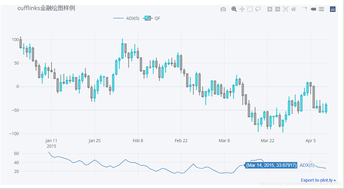
13.添加平均趋向指数ADX

import cufflinks as cf
cf.set_config_file(offline=True, world_readable=True)
qf=cf.QuantFig(df,title='cufflinks金融绘图样例',legend='top',name='QF')
qf.add_adx(periods=5)
qf.iplot()

效果图：

参数介绍：

"""
		Parameters:
			periods : int or list(int)
				Number of periods
			name : string
				Name given to the study
			str : string
				Label factory for studies
				The following wildcards can be used:
					{name} : Name of the column
					{study} : Name of the study
					{period} : Period used
				Examples:
					'study: {study} - period: {period}'
		kwargs: 
			legendgroup : bool
				If true, all legend items are grouped into a 
				single one
			All formatting values available on iplot()
		"""

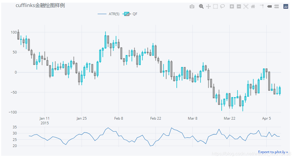
14.添加均幅指标ATR

import cufflinks as cf
cf.set_config_file(offline=True, world_readable=True)
qf=cf.QuantFig(df,title='cufflinks金融绘图样例',legend='top',name='QF')
qf.add_atr(periods=5)
qf.iplot()

效果图：

参数介绍：

"""
		Parameters:
			periods : int or list(int)
				Number of periods
			name : string
				Name given to the study
			str : string
				Label factory for studies
				The following wildcards can be used:
					{name} : Name of the column
					{study} : Name of the study
					{period} : Period used
				Examples:
					'study: {study} - period: {period}'
		kwargs: 
			legendgroup : bool
				If true, all legend items are grouped into a 
				single one
			All formatting values available on iplot()
		"""

15.添加趋向指标DMI

import cufflinks as cf
cf.set_config_file(offline=True, world_readable=True)
qf=cf.QuantFig(df,title='cufflinks金融绘图样例',legend='top',name='QF')
qf.add_dmi(periods=5)
qf.iplot()

效果图：

参数介绍：

"""
		Parameters:
			periods : int or list(int)
				Number of periods
			name : string
				Name given to the study
			str : string
				Label factory for studies
				The following wildcards can be used:
					{name} : Name of the column
					{study} : Name of the study
					{period} : Period used
				Examples:
					'study: {study} - period: {period}'
		kwargs: 
			legendgroup : bool
				If true, all legend items are grouped into a 
				single one
			All formatting values available on iplot()
		"""

拓展内容

1.剔除非交易日期

当我们使用自己的数据绘图时，其默认会把 非交易日也包含在图中。例如下面从tushare中获取数据：

import cufflinks as cf
import tushare as ts
cf.set_config_file(offline=True, world_readable=True)
df=ts.get_hist_data('000001',start='2020-04-15',end='2020-05-13')
qf=cf.QuantFig(df,title='cufflinks金融绘图样例',legend='top',name='QF')
qf.iplot()

效果图：

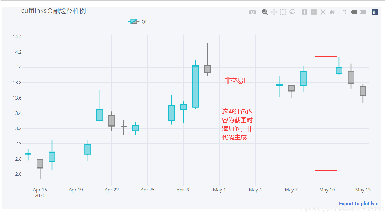
可以看到，绘制的图像包含了非交易日。如果我们想要剔除这些非交易日，需要把代码修改为：

import cufflinks as cf
import tushare as ts
cf.set_config_file(offline=True, world_readable=True)
df=ts.get_hist_data('000001',start='2020-04-15',end='2020-05-13')
qf=cf.QuantFig(df,title='cufflinks金融绘图样例',legend='top',name='QF')
layout = dict(
    xaxis=dict(
        categoryorder="category ascending",#筛除非交易日
        type='category')
)
qf.iplot(layout=layout)

效果图：

可以看到，在添加了layout后，图像底部多出了一个选择横坐标范围的小条。同时在layout中将xaxis的type设置为‘category’便可以剔除非交易日了。

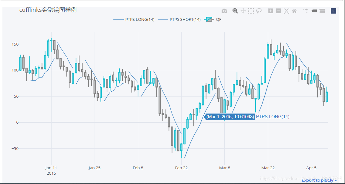
2.抛物转向指标add_ptps报错

除了上面介绍的方法外，cufflinks还有添加抛物转向指标add_ptps(),但我测试的时候，该方法一直报错。

import cufflinks as cf
cf.set_config_file(offline=True, world_readable=True)
df=cf.datagen.ohlcv()
qf=cf.QuantFig(df,title='cufflinks金融绘图样例',legend='top',name='QF')
qf.add_ptps()
qf.iplot()

错误最终指向：

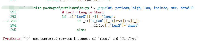
提示说是计算过程中出现了None。
初步考察，应该是cufflinks的源码的问题(如果不是还请大佬指出）
打开cufflinks中的ta.py文件

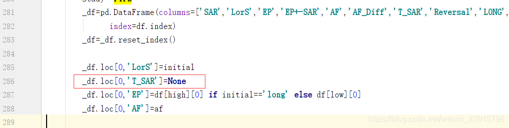
可以看到，在286行，其将某一单元的初值设置为None，而该单元恰好是在报错的位置出现的变量。
解决方法：注释掉286行。