信用卡异常交易识别
1.数据处理
1.1 数据集初始可视化与问题查询
数据集处理是机器学习中极其重要的一步,不同的测试集与训练集构建方法会对机器学习的效果带来巨大的影响。因此,常常在开始训练模型之前,我们就做好不同重点的测试集与训练集构建方法。
在处理数据集之前,可以针对感兴趣的变量进行初步的可视化(直方图、密度图、时许图等),并查询数据集存在的问题(数据分布有偏、量级差距过大、有缺失值等)
1.1.1 数据集查看与初始可视化
>>>data.head()
   Time        V1        V2        V3  ...       V27       V28  Amount  Class
0   0.0 -1.359807 -0.072781  2.536347  ...  0.133558 -0.021053  149.62      0
1   0.0  1.191857  0.266151  0.166480  ... -0.00898》3  0.014724    2.69      0
2   1.0 -1.358354 -1.340163  1.773209  ... -0.055353 -0.059752  378.66      0

# 查看Class分布
data['Class'].value_counts()
0    284315
1       492
Name: Class, dtype: int64

# 查看数据集中是否存在确实值
data.isnull().all()
data.isnull().any()

# 数据标签直方图
count_classes = pd.value_counts(data['Class'],sort = True).sort_index()
count_classes.plot(kind = 'bar')
plt.title('Fraud class histogram')
plt.xlabel('Class')
plt.ylabel('Frequency')
plt.show()
该数据集有包含Time在内的30个变量,其中Class中,0为正样本,1为负样本;
初步判断Time对本问题是不重要的变量,Amount变量与其他变量数量级差别过大,需进行标准化操作;
无缺失值;
正样本与负样本差距过大,考虑采取下采样、过采样两种训练集与测试集划分方式。
1.1.2 数据处理
针对在上一步得到的问题进行数据处理,标准化处理是常见的必须操作。
# 数据标准化处理
from sklearn.preprocessing import StandardScaler
data['normAmount'] = StandardScaler().fit_transform(data['Amount'].values.reshape(-1,1))
data = data.drop(['Time','Amount'],axis = 1)

>>>data.head()
         V1        V2        V3  ...       V28  Class  normAmount
0 -1.359807 -0.072781  2.536347  ... -0.021053      0    0.244964
1  1.191857  0.266151  0.166480  ...  0.014724      0   -0.342475
2 -1.358354 -1.340163  1.773209  ... -0.059752      0    1.160686
3 -0.966272 -0.185226  1.792993  ...  0.061458      0    0.140534
4 -1.158233  0.877737  1.548718  ...  0.215153      0   -0.073403
2.训练集与测试集的构建
测试集与训练集的不同构建方式会对模型结果产生非常大的影响。在划分数据集时,常见的流程是,先进行数据切片,在训练集中对模型进行训练,得到最优的模型之后,将该模型应用于测试集中进一步完善,最后将此模型应用于实践。
2.1 预备工作
将特征与标签、正样本与负样本区分开来,以便后续操作。同时设置好测试集。
X = data.iloc[:,data.columns!='Class']
y = data.iloc[:,data.columns =='Class']

positve_indices = np.array(data[data.Class==0].index)
negative_indices = np.array(data[data.Class ==1].index)

# 得到有效测试集X_test,y_test
X_train,X_test,y_train,y_test =  train_test_split(X,y,test_size=0.3,random_state = 0)
2.1 下采样方式
下采样方式是使得训练集中的正样本与负样本个数相同(削减正样本的数量)。
from sklearn.model_selection import train_test_split

# 随机抽样得到正样本索引
random_positive_indices = np.random.choice(positve_indices,len(negative_indices),replace = False)
# 得到下采样数据集索引
undersample_indices = np.array(list(random_positive_indices)+list(negative_indices)).flatten()

X_undersample = X.iloc[undersample_indices,:]
y_undersample = y.iloc[undersample_indices,:]

# 得到有效训练集X_undersample_train,y_undersample_train
X_undersample_train,X_undersample_test,y_undersample_train,y_undersample_test = train_test_split(X_undesample,y_undersample,test_size=0.3,random_state = 0)
有效训练集X_undersample_train,y_undersample_train用于训练模型
有效测试集y_test用于测试模型
为什么不用y_undersample_test来测试?首先,应当放到真实环境中去测试。其次,y_undersample_test中,正样本与负样本的个数比与原数据集的情况差别过大。
2.2 过采样方式
SMOTE方式是使得训练集中的正样本与负样本个数相同(增加负样本的数量)。
# 保证每一次生成的样本是一样的
oversampler = SMOTE(random_state=0)
# 从训练集中生成,使得数据集中正样本数量与负样本数量一致
os_features, os_labels = oversampler.fit_sample(X_train,y_train)

# 得到训练集os_features_train,os_labels_train
os_features_train,os_features_test,os_labels_train,os_features_test=train_test_split(os_features,os_features,test_size=0.3,random_state=0)

# 生成数据框方便矩阵运算
os_features_train = pd.DataFrame(os_features_train)
os_labels_train = pd.DataFrame(os_labels_train)
3.KFold交叉验证
3.1 K折交叉验证的流程
首先,在设定好测试集之后,就需要对其再次划分进行K折交叉验证。生成交叉验证的代码如下:
from sklearn.model_selection import KFold
# 交叉验证:在训练集中进一步拆分出训练集与验证集
# shuffle为False时,无须设置随机种子
fold = KFold(n_splits=5,shuffle=False)
fold = fold.split(X_train_data)

# 查看fold的输出结果,前者是测试集的index,后者是验证集的index
for iteration, indices in fold.split(X_train_data):
    print(iteration)
    print(indices)
接着,应将选择好的模型放入到K折交叉训练集之中进行训练。一次训练的代码如下(本项目使用逻辑回归进行分类):
# 指定算法模型,并且给定参数
lr = LogisticRegression(C = c_param,penalty='l1',solver='liblinear')

# 训练模型
lr.fit(X_train_data.iloc[iteration,:],y_train_data.iloc[iteration,:].values.ravel())

# 建立好模型后,预测模型结果,使用验证集
y_pred_undersample = lr.predict(X_train_data.iloc[indices,:].values)

# 有了预测结果之后就可以进行评估了
recall_acc = recall_score(y_train_data.iloc[indices,:].values,y_pred_undersample)
recall_accs.append(recall_acc)
最后,应将每次的结果进行平均,找到最适合的模型,将上述过程封装成函数为:
def printing_Kfold_scores(X_train_data,y_train_data):
    fold = KFold(n_splits=5,shuffle=True,random_state = 10)

    # 定义不同力度的正则化惩罚力度
    c_param_range = [0.01,0.1,1,10,100]
    # 生成一个储存结果的数据框
    results_table = pd.DataFrame(index = range(len(c_param_range),2),columns=['C_parameter','Mean recall score'])
    results_table['C_parameter'] = c_param_range
    j = 0
    for c in c_param_range:
        c_param = c
        print('--------------------------------------')
        print('正则化惩罚力度:',c)
        print('--------------------------------------')
        print('')
        s = 1
        recall_accs = []
        for iteration,indices in fold.split(X_train_data):
            # 指定好模型
            lr = LogisticRegression(C = c_param ,penalty='l1',solver='liblinear')
            # 使用训练集训练模型
            lr.fit(X_train_data.iloc[iteration,:],y_train_data.iloc[iteration,:].values.ravel())
            # 使用验证集进行验证
            y_pred = lr.predict(X_train_data.iloc[indices,:])
            # 评估预测结果
            recall_acc = recall_score(y_train_data.iloc[indices, :].values, y_pred)
            print('iteration:',s,'召回率为:',recall_acc)
            s = s+1
            recall_accs.append(recall_acc)
        # 执行完所有的交叉验证之后,计算平均值
        recall_accs_avg =np.mean(recall_accs)
        print('')
        print('平均召回率为:',recall_accs_avg)
        print('')
        results_table.iloc[j,1]=recall_accs_avg
        j = j+1
    # 找到最优模型
    best_c = results_table.loc[results_table['Mean recall score'].astype('float32').idxmax()]['C_parameter']
    print('*************************************************************')
    print('效果最好的模型所选参数=',best_c)
    print('*************************************************************')

    return best_c
下采样数据集结果:
--------------------------------------
正则化惩罚力度: 0.01
--------------------------------------
iteration: 1 召回率为: 0.9428571428571428
iteration: 2 召回率为: 0.9264705882352942
iteration: 3 召回率为: 0.9523809523809523
iteration: 4 召回率为: 0.953125
iteration: 5 召回率为: 0.9743589743589743
平均召回率为: 0.9498385315664727
--------------------------------------
正则化惩罚力度: 0.1
--------------------------------------
iteration: 1 召回率为: 0.9
iteration: 2 召回率为: 0.8529411764705882
iteration: 3 召回率为: 0.8888888888888888
iteration: 4 召回率为: 0.90625
iteration: 5 召回率为: 0.9230769230769231
平均召回率为: 0.89423139768728
--------------------------------------
正则化惩罚力度: 1
--------------------------------------
iteration: 1 召回率为: 0.9
iteration: 2 召回率为: 0.8676470588235294
iteration: 3 召回率为: 0.9365079365079365
iteration: 4 召回率为: 0.90625
iteration: 5 召回率为: 0.9102564102564102
平均召回率为: 0.9041322811175754
--------------------------------------
正则化惩罚力度: 10
--------------------------------------
iteration: 1 召回率为: 0.9285714285714286
iteration: 2 召回率为: 0.8823529411764706
iteration: 3 召回率为: 0.9365079365079365
iteration: 4 召回率为: 0.890625
iteration: 5 召回率为: 0.9102564102564102
平均召回率为: 0.9096627433024492
--------------------------------------
正则化惩罚力度: 100
--------------------------------------
iteration: 1 召回率为: 0.9285714285714286
iteration: 2 召回率为: 0.8970588235294118
iteration: 3 召回率为: 0.9365079365079365
iteration: 4 召回率为: 0.890625
iteration: 5 召回率为: 0.9102564102564102
平均召回率为: 0.9126039197730375
*************************************************************
效果最好的模型所选参数= 0.01
*************************************************************
SMOTE过采样方案结果:
--------------------------------------
正则化惩罚力度: 0.01
--------------------------------------
iteration: 1 召回率为: 0.9153998203054807
iteration: 2 召回率为: 0.9141990724224046
iteration: 3 召回率为: 0.9115085480807139
iteration: 4 召回率为: 0.9114050411779386
iteration: 5 召回率为: 0.9098122284852619
平均召回率为: 0.9124649420943598
--------------------------------------
正则化惩罚力度: 0.1
--------------------------------------
iteration: 1 召回率为: 0.917340521114106
iteration: 2 召回率为: 0.9166250445950767
iteration: 3 召回率为: 0.913909895702663
iteration: 4 召回率为: 0.9136867624514243
iteration: 5 召回率为: 0.9121459088787564
平均召回率为: 0.9147416265484052
--------------------------------------
正则化惩罚力度: 1
--------------------------------------
iteration: 1 召回率为: 0.9184905660377358
iteration: 2 召回率为: 0.9170174812700678
iteration: 3 召回率为: 0.9143399878140569
iteration: 4 召回率为: 0.9147919711932689
iteration: 5 召回率为: 0.9129716727103006
平均召回率为: 0.9155223358050861
--------------------------------------
正则化惩罚力度: 10
--------------------------------------
iteration: 1 召回率为: 0.9178796046720575
iteration: 2 召回率为: 0.9170888333927935
iteration: 3 召回率为: 0.9144116698326225
iteration: 4 召回率为: 0.9147919711932689
iteration: 5 召回率为: 0.912325422755179
平均召回率为: 0.9152995003691844
--------------------------------------
正则化惩罚力度: 100
--------------------------------------
iteration: 1 召回率为: 0.9187061994609165
iteration: 2 召回率为: 0.917160185515519
iteration: 3 召回率为: 0.9148417619440163
iteration: 4 召回率为: 0.9148989268779636
iteration: 5 召回率为: 0.9124331310810325
平均召回率为: 0.9156080409758897
*************************************************************
效果最好的模型所选参数= 100.0
*************************************************************
可以看到,针对不同的数据方式,其得到的结果可能会产生非常的差异。
3.2 K折交叉验证模型结果的可视化
针对分类问题有许多模型效果评估指标,比如混淆矩阵,ROC,AUC等等。这里仅使用混淆矩阵作为示范。
import itertools

def plot_confusion_matrix(cm,classes,title = 'Confusion matrix', cmap = plt.cm.Blues):
    plt.imshow(cm,interpolation='nearest',cmap = cmap)
    plt.title(title)
    plt.colorbar()
    tick_marks = np.arange(len(classes))
    plt.xticks(tick_marks,classes,rotation = 0)
    plt.yticks(tick_marks,classes)

    thresh = cm.max()/2
    for i,j in itertools.product(range(cm.shape[0]),range(cm.shape[1])):
        plt.text(j,i,cm[i,j],
                 color = 'white'
                 if cm[i,j]>thresh
                 else 'black')
    plt.tight_layout()
    plt.ylabel('True label')
    plt.xlabel('Predicted label')
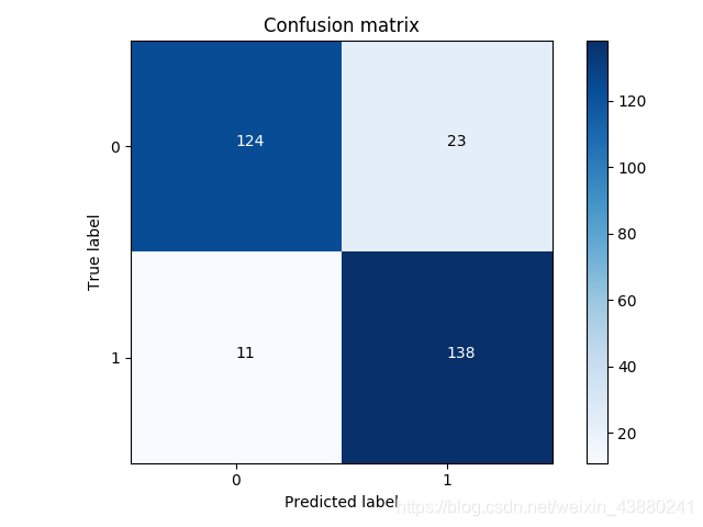
下采样方法的混淆矩阵
class_names = [0,1]
lr = LogisticRegression(C=best_c1,penalty='l1',solver='liblinear')
lr.fit(X_undersample_train,y_undersample_train.values.ravel())
y_pred_undersample = lr.predict(X_undersample_test.values)
cnf_matrix = confusion_matrix(y_undersample_test,y_pred_undersample)
np.set_printoptions(precision =2)
plot_confusion_matrix(cnf_matrix,classes=class_names,title = 'Confusion matrix')
plt.show()
SMOTE过采样方法的混淆矩阵

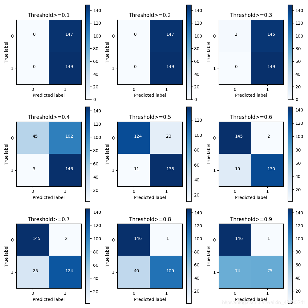
4.问题查询
可以从混淆矩阵中找到合适的阈值,来影响分类效果。
# 阈值对结果的影响
lr = LogisticRegression(C=0.01,penalty='l1',solver='liblinear')

# 训练模型
lr.fit(X_train_undersample,y_train_undersample.values.ravel())

# 为了控制阈值,因此返回概率值
y_pred_undersample_proba = lr.predict_proba(X_test_undersample.values)

# 指定不同的阈值
thresholds = [0.1,0.2,0.3,0.4,0.5,0.6,0.7,0.8,0.9] #0.4稍微异常就被抓,0.9非常有可能是的时候才抓起来
plt.figure(figsize=(10,10))
j=1
# 用混淆矩阵来进行展示
for i in thresholds:
    y_test_predictions_high_recall = y_pred_undersample_proba[:,1]>i
    plt.subplot(3,3,j)
    j +=1

    cnf_matrix = confusion_matrix(y_test_undersample,y_test_predictions_high_recall)
    np.set_printoptions(precision = 2)
    print('给定阈值为:',i,'时测试集召回率:',cnf_matrix[1,1]/(cnf_matrix[1,0]+cnf_matrix[1,1]))

    class_names = [0,1]
    plot_confusion_matrix(cnf_matrix,
                          classes=class_names,
                          title='Threshold>=%s'%i)
plt.show()
参考:唐宇迪python实战课;周志华《机器学习》
