强化学习入门笔记
- Concepts in Reinforcement Learning
- Difficulties in RL
- A3C Method Brief Introduction
- Policy-based Approach - Learn an Actor (Policy Gradient Method)
- 1. Decide Function of Actor Model (NN? ...)
- 2. Decide Goodness of this Function
- 3. Choose the best function
- On-Policy v.s. Off-Policy
- Importance Sampling (On-Policy Off-Policy)
- PPO Algorithm —— Proximal Policy Optimization
- Value-based Approach - Learn an Critic
- A3C Method - Asynchronous Advantage Actor-Critic
- Sparse Reward
Concepts in Reinforcement Learning
- The main goal of Reinforcement Learning is to maximum the
Total Reward. Total Rewardis the sum of all reward inOne Eposide, so the model doesn’t know which steps in this episode are good and which are bad.- Only few actions can get the positive reward (ex: fire and killing the enemy in Space War game gets positive reward but moving gets no reward), so how to let the model find these right actions is very important.
Difficulties in RL
- Reward Delay
- Only “Fire” can obtain rewards, but moving before fire is also important (moving has no reward), how to let the model learn to move properly?
- In chess game, it may be better to sacrifice immediate reward to gain more long-term reward.
- Agent’s actions may affect the environment
- How to explore the world (
observation) as more as possible. - How to explore the
action-combinationas more as possible.
- How to explore the world (
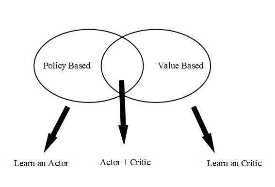
A3C Method Brief Introduction
The A3C method is the most popular model which combines policy-based method and value-based method, the structure is shown as below. To learn A3C model, we need to know the concepts of policy-based and value-based. The details of A3C are shown [here](#A3C Method - Asynchronous Advantage Actor-Critic).
Policy-based Approach - Learn an Actor (Policy Gradient Method)
This approach try to learn a policy(also called actor). It accepts the observation as input, and output an action. The policy(actor) can be any model. If you an Neural Network to as your actor, then you are doing Deep Reinforcement Learning.
There are three steps to build DRL:
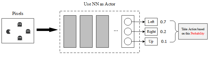
1. Decide Function of Actor Model (NN? …)
Here we use the NN as our Actor, so:
- The Input of this NN is the observation of machine represented as Vector or Matrix. (Ex: Image Pixels to Matrix)
- The Output of this NN is Action
Probability. The most important point is that we shouldn’t always choose the action which has the highest probability, it should be a stochastic decisions according to the probability distribution. - The Advantage of NN to Q-table is: we can’t enumerate all observations (such as we can’t list all pixels’ combinations of a game) in some complex scenes, then we can use Neural Network to promise that we can always obtain an output even if this observation didn’t appear in the previous train set.
2. Decide Goodness of this Function
Since we use the Neural Network as our function model, we need to decide what is the goodness of this model (a standard to judge the performance of current model). We use to express this standard, which is the parameters of current model.
- Given an actor with Network-Parameters , is the observation (input).
- Use the actor to play the video game until this game finished.
- Sum all rewards in this episode and marked as
.
Note: is a variable, cause even if we use the same actor to play the same game many times, we can get the different (random mechanism in game and action chosen). So we want to maximum the which expresses the expect of . - Use the to expresses the goodness of .
How to Calculate the ?
-
An episode is considered as a trajectory
- = { } all the history in this episode
-
Different has different probability to appear, the probability of is depending on the parameter of actor . So we define the probability of as .
-
We use actor to play N times game, obtain the list { }. Each has a reward , the mean of these approximate equals to the expect .
3. Choose the best function
Now we need to know how to calculate the
, here we use the Gradient Ascend method.
- problem statements:
- gradient ascent:
- Start with .
- …
- The includes the parameters in the current Neural Network, $\theta = $ { }, which the .
It’s time to calculate the gradient of , since has nothing to do with , the gradient can be expressed as:
Note:
Use
policy play the game N times, obtain {
}:
How to Calculate the ?
Since
is the history of one episode, so:
KaTeX parse error: No such environment: align* at position 8: \begin{̲a̲l̲i̲g̲n̲*̲}̲ P(\tau|\theta)…
Ignore the terms which not related to :
So the final result of is :
The meaning of this equation is very clear:
- if is positive tune to increase the .
- if is negative tune to decrease the
Use this method can resolve the [Reward Delay Problem](#Difficulties in RL) in Difficulties in RL chapter, because here we use the cumulative reward of one entire episode
, not just the immediate reward after taking one action.
Add a Baseline - b
To avoid all of
is positive (there should be some negative reward to tell model don’t take this action at this state), we can add a baseline. So the equation changes to:
Assign Suitable Weight of each Action
Use the total reward to tune the all actions’ probability in this episode also has some disadvantage, show as below:
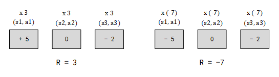
The left picture show one episode whose total reward R is 5, so the probabilities of all actions in this episode will be increased (such as x5), but the main positive reward obtained from the , while and didn’t give any positive reward, but the probability of and also be increased in this example. Same as right picture, is a bad action, but may not be a bad action, so probability of shouldn’t be decreased.
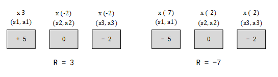
To avoid this problem, we assign different to each , the is the cumulation of which is the sum of all rewards obtained after , now the equation becomes:
Note:
called discount factor,
.
We can use
to express the
in above equation, which called Advantage Function. This function evaluate how good it is if we take
at this state
rather than other actions.
On-Policy v.s. Off-Policy
On-Policy and Off-Policy are two different modes of learning:
- On-Policy: The agent learn the rules by
interactingwith environment. (learn from itself) - Off-Policy: The agent learn the rules by
watchingothers’ interacting with environment. (learn from others)
Our Policy Gradient Method is an On-Policy learning mode, so why we need Off-Policy mode? This is because we use sampling N times and get the mean value to approximate the expect . But when we update the , the changed, so we need to do N sampling again and get the mean value. This will take a lot of time to do sampling after we update . The resolution is, we build a model , this model accept the training data from the other model . Use to collect data, and train the with , since don’t change , the sampling data can be reused.
Importance Sampling (On-Policy Off-Policy)
Importance Sampling is a method to get the expect of one function by sampling another function . Since we have already known:
But if we only have { } sampled from , how to use this samples to calculate the ? We can change equation above:
That means we can get the expect of distribution
by sampling the {
} from another distribution
, only need to do some rectification,
called rectification term. Now we can consider our
model as
, the
as
, use the
to sample data to tune
.
then we can use to sample many times and train many times. After many iterations, we update . Continue to transform the equation:
Let the , and . We consider the environment observation is not related to actor (ignore the environment changing by action), then , equation becomes:
Here defines:
Note: Since we use
to sample data for
, the distribution of
can’t be very different from
, how to determine the difference between two distribution and end the model training if
is distinct from
? Now let’s start to learn PPO Algorithm.
PPO Algorithm —— Proximal Policy Optimization
PPO is the resolution of above question, it can avoid the problem which raised from the difference between
and
. The target function shows as below:
which the
is the divergence of output action from policy
and policy
. The algorithm flow is:
-
Initial Policy parameters
-
In each iteration:
- Using to interact with the environment, and collect { } to calculate the
-
Update the several times: $ J_{PPO}{\thetak}(\theta) = J{\thetak}(\theta) - \beta KL(\theta, \theta^k)$
-
If , that means KL part takes too big importance of this equation, increase
-
If , that means KL part takes lower importance of this equation, decrease
Value-based Approach - Learn an Critic
A critic doesn’t choose an action (it’s different from actor), it evaluates the performance of a given actor. So an actor can be found from a critic.
Q-learning
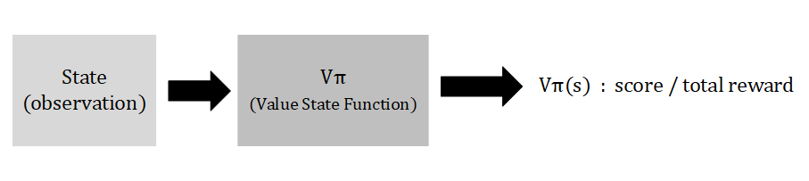
Q-Learning is a classical value-based method, it evaluates the score of an observation under an actor
, this function is called state value function
. The score is calculated as the total reward from current observation to the end of this episode.
How to estimate ?
We know we need to calculate the total reward to express the performance of current actor , but how to get this value?
- Monte-Carlo based approach
In the current state (observation), until the end of this episode, the cumulated reward is ; In the current state (observation), until the end of this episode, the cumulated reward is . That means we can estimate the value of an observation under an actor , the low value could be explain as two possibilities:
a) the current observation is bad, even if a good actor can not get a high value.
b) the actor has a bad performance.
In many cases, we can’t enumerate all observations to calculate the all rewards . The resolution is using a Neural-Network to fit the function from observation to value .
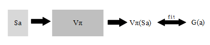
Fit the NN with , try to minimize the difference between the NN output and Monte-Carlo reward .
- Temporal-Difference approach
MC approach is worked, but the problem is you must get the total reward in the end of one episode. It may be a very long way to reach the end state in some cases, Temporal-Difference approach could address this problem.
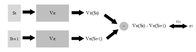
here is a trajectory { }, there should be:
so we can fit the NN by minimize the difference between and .
Here is a tip in practice: we are training the same model , so the two outputs and are all generate from one parameter group . When we update the after one iteration, both and are changed in next iteration, which makes the model unstable.
The tip is: fix the parameter group to generate the , and update the for . After N iterations, let the equal to . Fixed parameter Network (right) is called Target Network.
-
MC v.s. TD
- Monte-Carlo has larger
variance. This is caused by the randomness of , since is the sum of all reward , each is a random variable, the sum of these variable must have a larger variance. Playing N times of one game with the same policy, the reward set { } has a large variance. - Temporal-Difference also has a problem, which is
may estimate
incorrectly(cause it’s not like Monte-Carlo approach to cumulative the reward until the end of this episode), so even the is correct, the may not correct.
In the practice, people prefer to use TD method.
- Monte-Carlo has larger
-
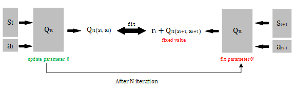
Q-value approach
In current state (observation), enumerate all valid actions and calculate the Q-value of each action.
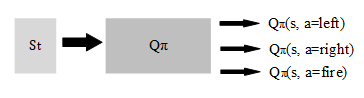
note: In current state we force the actor to take the specific action to calculate the value this action, but random choose actions according to the
actor in next steps until the end of episode.
Use Q-value to learn an actor
We can learn an actor with the Q-value function, here is the algorithm flow:
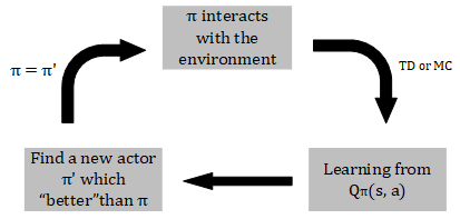
If is better than , then:
We can use equation below to calculate the
from
:
Note: This approach not suitable for continuous action, only for discrete action.
But if we always choose the best action according to the
, some other better actions we can never detect. So we infer use Exploration method when we choose action to do.
Epsilon Greedy
Set a probability
, take max Q-value action or take random action show as below. Typically ,
decreases as time goes by.
KaTeX parse error: No such environment: align at position 20: … \left\{ \begin{̲a̲l̲i̲g̲n̲}̲ argmaxQ(s, a)&…
Boltzmann Exploration
Since the
is an Neural Network, the output of this Network is the probability of each action. Use this probability to decide which action should take, show as below:
Q-value may be negative, so we take exp-function to let them be positive.
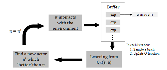
Replay Buffer
Replay buffer is a buffer which stores a lot of experience data. When you train your Q-Network, random choose a batch from buffer to fit it.
-
An experience is a set which looks like { }.
-
The experience in buffer may comes from different policy { }.
-
Drop the old experience when buffer is full.
Typical Q-Learning Algorithm
Here is the main algorithm flow of Q-learning:
- Initialize Q-function Q, Initialize target Q-function
- in each episode
- for each step t
- Given state , take an action based on Q ( -greedy exploration)
- Obtain the reward and next state
- Store this experience { } into the replay buffer
- Sample a batch of experience { } from buffer
- Compute target
- Update the parameters in to make close to .
- After N steps set
- for each step t
Double DQN
Double DQN is designed to solve the problem of DQN. Problem of DQN show as below:
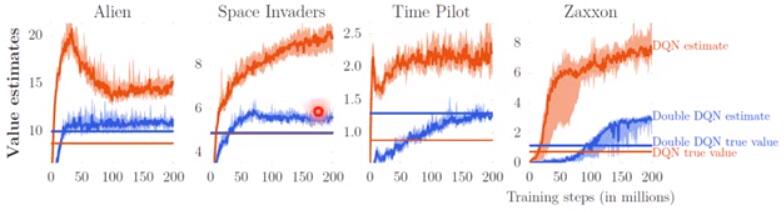
Q-value are always over estimate in DQN training (Orange curve is DQN Neural Network output reward, Blue curve is Double DQN Neural Network output reward; Orange line is the real cumulative reward of DQN, Blue line is the real cumulative reward of Double DQN). Notes that Blue lines are over than Orange lines which means Double DQN has a greater true value than DQN.
Why DQN always over-estimate Q-value?
This because when we calculate the target
which equals
, we always choose the best action and compute the highest Q-value. This may over-estimate the target value, so the real cumulative reward may lower than that target value. While Q function is try to close the target value, this results the output of Q-Network is higher than the actual cumulative reward.
Double DQN resolution
To avoid above problem, we use two Q-Network in training, one is in charge of choose the best action and the other is to estimate Q-value.
Here use
to select the best action in each state but use
to estimate the Q-value of this action. This method has two advantages:
- If over-estimate the Q-value of action , although this action is selected, the final Q-value of this action won’t be over estimated (because we use to estimate the Q-value of this action).
- If over-estimate one action , it’s also safe. Because the policy won’t select the action (because is not the best action in Policy ).
In DQN algorithm, we already have two Network: origin Network
and target Network
(need to be fixed). So here use origin Network $\theta $ to select the action, and target Network $\theta’ $ to estimate the Q-value.
Other Advanced Structure of Q-Learning
- Dueling DQN
Change the output as two parts: , which means the final Q-value is the sum of environment value and action value.
- Prioritized Replay
When we sample a batch of experience from replay buffer, we don’t use random select. Prioritized Replay marked those experience which has a high loss after one iteration, and increase the probability of selecting those experience in the next batch.
- Multi-Step
Change the experience format in the Replay Buffer, not only store one step {$ s_t, a_t, r_t, s_{t+1} $}, store N steps { }.
- Noise Net
This method used to explore more action. Add some noise in current Network at the beginning of one episode.
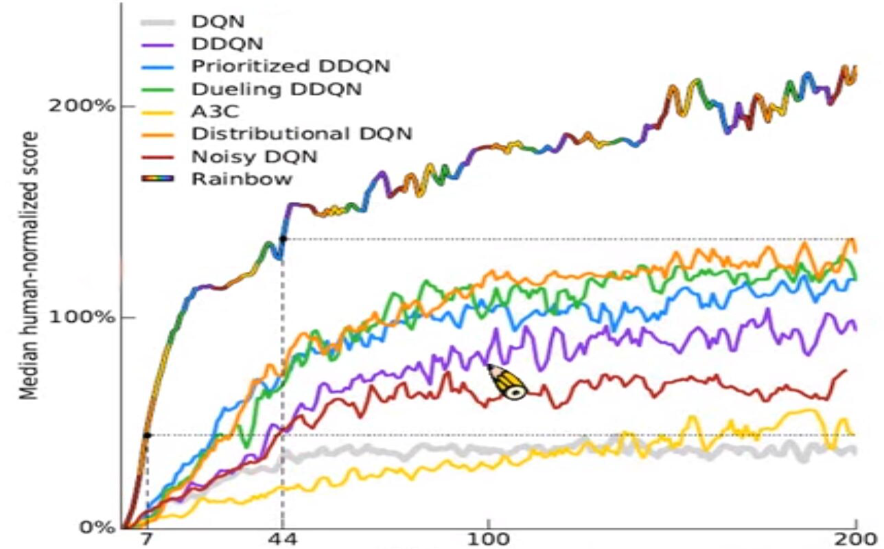
Here is the comparison of different algorithms:
A3C Method - Asynchronous Advantage Actor-Critic
Why we need A3C method? This is designed to solve the variance problem of Policy Gradient. In Policy Gradient method, even in the same state $ s_t $ and take the same action $ a_t $ N times, we may get very different result total reward
. This because randomness existed when we calculate the cumulative reward in below equation:
This part $ (\sum_{t’=t}T{\gamma{t’ -t}r_{t’}^n} - b) $ could be very different for $ r_t $ is a random variable with big variance, the result may be like this:
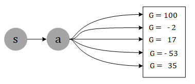
unless we sample enough times to cover all possible rewards, the model could be stable —— but it’s hard to do this. If we can replace
with the expect
, then we can solve this problem.
Advantage Actor-Critic (A2C Method)
We have already introduced value-based method, the definition of
is the expect of total reward of taking action
at current state
. The definition of $ V^{\pi_\theta}(s_t) $ is the expect reward of current state
(just the state value without specific which action should take). Now we change the equation:
note: Here we use state value to replace the baseline b.
We can infer the value of
from
:
We should use the expect because
is a random variable, but it’s hard to calculate, so we take off the expect. Now the equation becomes:
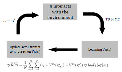
Algorithm flow of Advantage Actor-Critic method show as below:
Tips
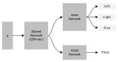
- There are two Networks to train in this algorithm: Actor $ \pi_\theta $ and Critic . But two networks accept the same input , only different in output —— scaler for Critic Network and Probability Distribution for Actor Network. So two networks can share some layers in the front of structure, looks like this:
- Use output entropy as regularization for , this could make the probability of each action more even so that the model can do more exploration.
Asynchronous Advantage Actor-Critic (A3C Method)
A3C is designed to speed up A2C. It maintain one global Network and create N workers, each worker interact with different environment, calculate the gradient and update the global Network.
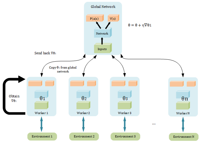
- Copy global parameters
- Sampling some data
- Compute gradients
- Update global model
note: All workers are parallelized, which means when
finish compute and send back to global model,
may changed (updated by other worker, so it may not remain $\theta_1 $). But we still use the
to update the current parameters
.
Sparse Reward
In reinforcement learning, reward is very important for agent to know which actions are good. But only few action could obtain a positive reward (ex. only fire and destroy the enemy could obtain a positive reward in Spaceship game), most of actions have no reward (ex. move left or move right). This phenomenon is called Sparse Reward.
Reward Shaping
Typically, few state could get the positive reward in training, thus we can create some extra rewards to guide the agent do some action in current state. For example, if we want to train an plane agent to destroy the enemy plane, the actual reward should be obtained from “fire and destroy the enemy”. But in the start of the game, our plane don’t know how to find enemy, so we can create an extra positive reward if our plane is fly toward enemy plane.
note: This method needs domain knowledge to design which rules desire positive reward and how much reward should be assigned.
Curriculum Learning
Typically, a hard task could be split into many simple tasks. Curriculum Learning Algorithm is starting from simple training examples, and then becoming harder and harder.
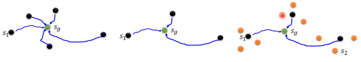
The most common technique is Reverse Curriculum Learning, explain as below:
- Given a goal state .
- Sample some states { } close to $s_g $.
- Each state has a reward to goal state , compute { }.
- Delete those state whose reward is too large (it’s too easy from this state to goal state) or too small (it’s too difficult from this state to goal state).
- Sample more states near the {$s_1, s_2, … }.
Hierarchical Reinforcement Learning
A entire model could be split into different hierarchies, top-level model only give the top-level order and low-level model choose the actual actions. For example, if we wanna train a plane agent, top-level model only give the way point of next target while the low-level model control the plane to fly to that target (turn left or turn right).
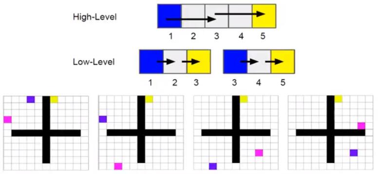
Here is a game example, blue point is the agent which is asked to reach the yellow point. Pink point is the temporary target given by high-level model while the low-level mode follow this instruction and control the agent to reach pink point.
ICM —— Intrinsic Curiosity Module
ICM Algorithm can let model to do more exploration. It adds an extra Reward function which accept three parameters . The Network need to maximize the sum value .
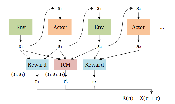
Now let’s see how ICM calculate reward in each step :
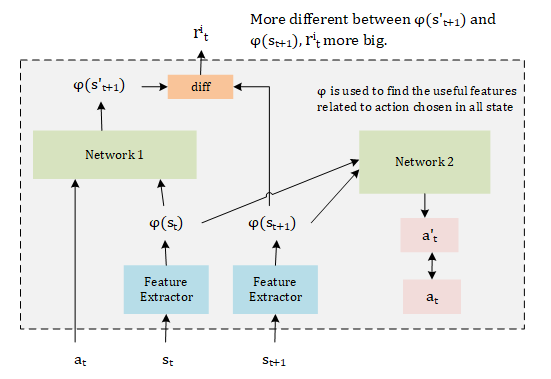
Here are two Networks in ICM module:
- Network 1: This Network is used to predict the next state after taking action , if is hard to predict, then the reward is high.
- Network 2: There may be a lot of features are not related to do actions (ex. the position of sun in the Spaceship War game). If we just maximize the reward of state which hard to predict, then the agent will stay and watch the sun moving. So we need to find the useful features in action chosen, this is the work of Network 2. It predict the action $a_t $ according to and .
