从TensorFlow2.0开始集成了Keras，变为了tensorflow.keras模块，其中，原Keras框架的一些方法已经丢弃，为了快速上手Keras，实现工程部署，从本篇文章开始更新基于TensorFlow 2.1.0的Keras使用系列教程。教程以小白视角编写，重要语句都做了注释。本文是该系列教程的第一篇。通过 Fashion MNIST 数据集实现图像分类，熟悉TensorFlow和Keras的建模流程和基本用法。

代码环境：

python version: 3.7.6 (default, Jan  8 2020, 20:23:39) [MSC v.1916 64 bit (AMD64)]
tensorflow version: 2.1.0

注：本文所有代码在 jupyter notebook 中编写并测试通过。

文章目录

1.Fashion MNIST 数据集
2. 数据可视化与预处理
3. 建模

3.1 定义模型
3.2 编译模型
3.3 训练模型
3.4 评估模型

4. 查看预测结果

4.1 测试集预测
4.2 预测结果可视化
4.3 单张图片预测

1.Fashion MNIST 数据集

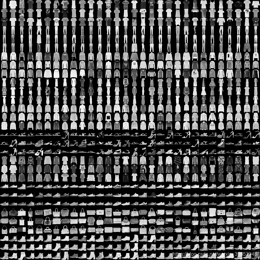
Fashion MNIST数据集包含10个类别的70,000张灰度图像。下图显示了低分辨率（28 x 28像素）的单个衣物：
在这里插入图片描述
Fashion MNIST旨在替代经典MNIST数据集，通常被用作计算机视觉机器学习程序的“ Hello，World”。这两个数据集用于验证算法是否按预期工作，是测试和调试代码的benchmark。本文例子使用60,000张图像训练网络，使用10,000张图像评估网络学习图像分类的准确率。直接从TensorFlow导入和加载Fashion MNIST数据：

导入表要的包：

import sys
import tensorflow as tf
from tensorflow import keras
print('python version:',sys.version)
print('tensorflow version:',tf.__version__)

加载数据集：

fashion_mnist = keras.datasets.fashion_mnist
(train_images, train_labels), (test_images, test_labels) = fashion_mnist.load_data()
# load_data()方法的返回值为：Tuple of Numpy arrays: (x_train, y_train), (x_test, y_test)

Fashion MNIST 中的图像是28x28 NumPy数组，像素值范围是0到255。标签是整数数组，范围是0到9，分别对应于图像表示的衣服真实标签为：

Label	Class
0		T-shirt/top
1		Trouser
2		Pullover
3		Dress
4		Coat
5		Sandal
6		Shirt
7		Sneaker
8		Bag
9		Ankle boot

原数据集中不包含真实标签，为方便绘图，首先用一个列表保存真实标签：

class_names = ['T-shirt/top', 'Trouser', 'Pullover', 'Dress', 'Coat',
               'Sandal', 'Shirt', 'Sneaker', 'Bag', 'Ankle boot']

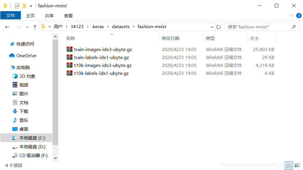
注意：在下载数据集的时候，可能会出现下载不全导致报错：【EOFError: Compressed file ended before the end-of-stream marker was reached】。解决方法：删除路径下对应的数据集文件之后，重新下载即可，比如我的在：【C:\Users\34123.keras\datasets】。无需科学上网，否则报SSL错误。下载比较慢或者卡死的话，直接从github下载，然后放到该路径下：
在这里插入图片描述

2. 数据可视化与预处理

1.基本信息

train_images.shape
#（60000，28，28）

train_labels
#array([9, 0, 0, ..., 3, 0, 5], dtype=uint8)

len(train_labels)
# 60000

len(test_labels)
# 10000

2.在训练网络之前，必须对数据进行预处理。检查训练集中第一张图像的像素值：

plt.figure()
plt.imshow(train_images[0])
plt.colorbar()
plt.grid(False)
plt.show()

在这里插入图片描述

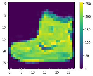
可以看到，其像素值落在0到255之间。
[1] matplotlib.pyplot.colorbar 官方文档

3.将这些值除以255，缩放到0到1，然后再将其输入神经网络模型。

train_images = train_images / 255.0
test_images = test_images / 255.0

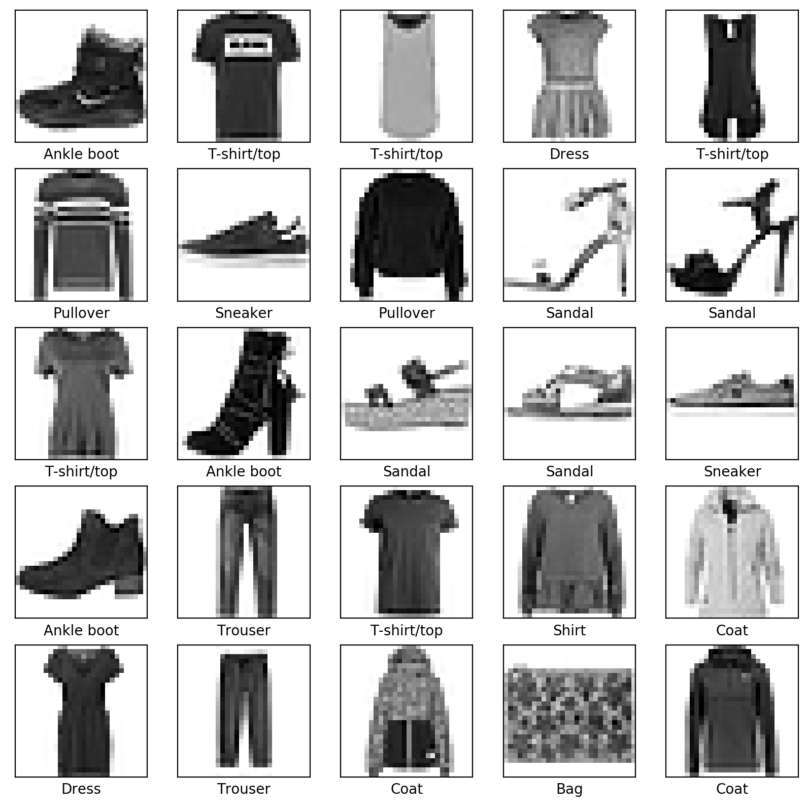
4.为了验证数据的格式正确，显示训练集中的前25个图像，并在每个图像下方显示类别名称：

plt.figure(figsize=(10,10), dpi=200)
for i in range(25):
    plt.subplot(5,5,i+1)
    plt.xticks([]) # 屏蔽坐标显示，下同
    plt.yticks([])
    plt.grid(False)
    plt.imshow(train_images[i], cmap=plt.cm.binary)
    plt.xlabel(class_names[train_labels[i]])
plt.show()

在这里插入图片描述

3. 建模

3.1 定义模型

model = keras.Sequential([
    keras.layers.Flatten(input_shape=(28, 28)),
    keras.layers.Dense(128, activation='relu'),
    keras.layers.Dense(10)
])

该网络的第一层 tf.keras.layers.Flatten 将图像格式从二维数组（28 x 28像素）转换为一维数组（28 * 28 = 784像素）。可以将这一层看作是堆叠图像中的像素行并将它们排成一行。该层没有学习参数，只会格式化数据。

像素展平后，添加两层 tf.keras.layers.Dense 层，即全连接层。第一个Dense层有128个节点（或神经元）。第二层（也是最后一层，即输出层）返回长度为 10 的logits数组。每个节点包含一个得分，指示当前图像属于10个类别中的哪一类。

3.2 编译模型

在训练模型之前，需要进行一些其他设置。这些是在模型的编译步骤中添加的：

优化器：基于模型看到的数据及其损失函数来更新模型的方式，即权重更新方式。
损失函数：衡量模型在训练过程中的准确性。训练过程即为最小化损失函数的过程。
指标：用于监视训练和测试过程。本例使用准确率为指标（正确分类的图像分数）。

model.compile(optimizer='adam',
              loss=tf.keras.losses.SparseCategoricalCrossentropy(from_logits=True),
              metrics=['accuracy'])

3.3 训练模型

训练神经网络模型需要执行以下步骤：

将训练数据输入模型（fit）。本例中，训练数据为train_images和train_labels组成的数组。
模型学习关联图像和标签。
配置模型对测试集进行预测（本例为test_images数组）。
验证预测是否与test_labels数组中的标签匹配。

model.fit(train_images, train_labels, epochs=10)

输出：

Train on 60000 samples
Epoch 1/10
60000/60000 [==============================] - 8s 128us/sample - loss: 0.4929 - accuracy: 0.8267
Epoch 2/10
60000/60000 [==============================] - 5s 89us/sample - loss: 0.3701 - accuracy: 0.8675
Epoch 3/10
60000/60000 [==============================] - 5s 86us/sample - loss: 0.3331 - accuracy: 0.8773
Epoch 4/10
60000/60000 [==============================] - 5s 91us/sample - loss: 0.3099 - accuracy: 0.8868
Epoch 5/10
60000/60000 [==============================] - 5s 87us/sample - loss: 0.2930 - accuracy: 0.8926
Epoch 6/10
60000/60000 [==============================] - 5s 83us/sample - loss: 0.2792 - accuracy: 0.8964
Epoch 7/10
60000/60000 [==============================] - 5s 88us/sample - loss: 0.2673 - accuracy: 0.9010
Epoch 8/10
60000/60000 [==============================] - 5s 88us/sample - loss: 0.2565 - accuracy: 0.9046
Epoch 9/10
60000/60000 [==============================] - 5s 87us/sample - loss: 0.2461 - accuracy: 0.9075
Epoch 10/10
60000/60000 [==============================] - 5s 90us/sample - loss: 0.2392 - accuracy: 0.9112
<tensorflow.python.keras.callbacks.History at 0x17b19ed3948>

模型训练时，会打印损失和准确率指标。该模型在训练数据上达到约91％（0.9112）的精度。

3.4 评估模型

接下来，比较模型在测试数据集上的表现：

test_loss, test_acc = model.evaluate(test_images,  test_labels, verbose=2)
print('\nTest accuracy:', test_acc)

输出：

10000/10000 - 1s - loss: 0.3307 - accuracy: 0.8846
Test accuracy: 0.8846

事实证明，测试数据集的准确性略低于训练数据集的准确性。训练准确性和测试准确性之间的差距表示出现了过拟合。当机器学习模型在新的输入数据上的表现比训练数据上的表现差时，即认为发生了过拟合。过拟合的模型“存储”训练数据集中的噪声和细节，从而对新数据的模型性能产生负面影响。有关更多欠拟合和过拟抑制策略，下篇介绍。

4. 查看预测结果

训练模型可以预测某些图像。模型的输出为线性的logits。通过softmax层可以将logits转换为更容易解释的概率。【注：对数 (logits)：分类模型生成的原始（非标准化）预测向量，通常会传递给标准化函数。如果模型要解决多类别分类问题，则对数通常变成 softmax 函数的输入。之后，softmax 函数会生成一个（标准化）概率向量，对应于每个可能的类别。】

4.1 测试集预测

添加softmax层实现分类概率预测：

probability_model = tf.keras.Sequential([model, tf.keras.layers.Softmax()])
predictions = probability_model.predict(test_images)

预测：

predictions[0]

输出：

array([6.1835679e-09, 5.0825996e-11, 1.7550703e-10, 1.2875578e-15,
       5.0945664e-11, 1.6961206e-04, 6.4031923e-08, 3.5876669e-03,
       1.0340054e-08, 9.9624264e-01], dtype=float32)

预测是10个数字组成的数组，表示模型对图像对应于10种不同服装中的每一种的置信度。查看置信度最高的标签：

np.argmax(predictions[0])

输出：

即模型对测试集中第一张图片的预测为标签 9，其对应的真实标签为 Ankle boot。

4.2 预测结果可视化

查看真实图片与预测：

def plot_image(i, predictions_array, true_label, img):
    '''
    该函数实现打印预测的图片
    '''
    predictions_array, true_label, img = predictions_array, true_label[i], img[i]
    plt.grid(False)
    plt.xticks([]) # 屏蔽坐标显示，下同
    plt.yticks([])

    plt.imshow(img, cmap=plt.cm.binary)

    predicted_label = np.argmax(predictions_array) # 取出预测最大概率的标签
    
    if predicted_label == true_label:
        color = 'blue'
    else:
        color = 'red'

    plt.xlabel("{} {:2.0f}% ({})".format(class_names[predicted_label], # 打印预测标签
                            100*np.max(predictions_array), # 打印置信度
                            class_names[true_label]), # 打印真实标签
                            color=color)

def plot_value_array(i, predictions_array, true_label):
    '''
    该函数实现绘制概率柱状图
    '''
    predictions_array, true_label = predictions_array, true_label[i]
    
    plt.grid(False) # 屏蔽格线显示
    plt.xticks(range(10))
    plt.yticks([]) 
    thisplot = plt.bar(range(10), predictions_array, color="#777777") # 绘制柱状图
    plt.ylim([0, 1]) # 设置y轴刻度显示范围
    
    predicted_label = np.argmax(predictions_array) # 取出预测标签

    thisplot[predicted_label].set_color('red') # 设置柱状图中预测标签的颜色
    thisplot[true_label].set_color('blue') 
    
def merged_result(i):
    '''
    该函数实现汇总以上两个函数输出结果，提供预测某张照片索引的接口
    '''
    plt.figure(figsize=(6,3), dpi=150)
    plt.subplot(1,2,1)
    plot_image(i, predictions[i], test_labels, test_images)
    plt.subplot(1,2,2)
    plot_value_array(i, predictions[i],  test_labels)
    plt.show()

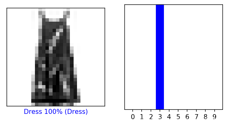
预测：

i = 12
merged_result(i)

在这里插入图片描述

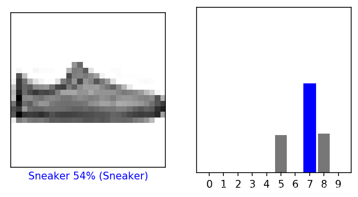
i = 450
merged_result(i)

输出：
在这里插入图片描述
输出多个预测结果：

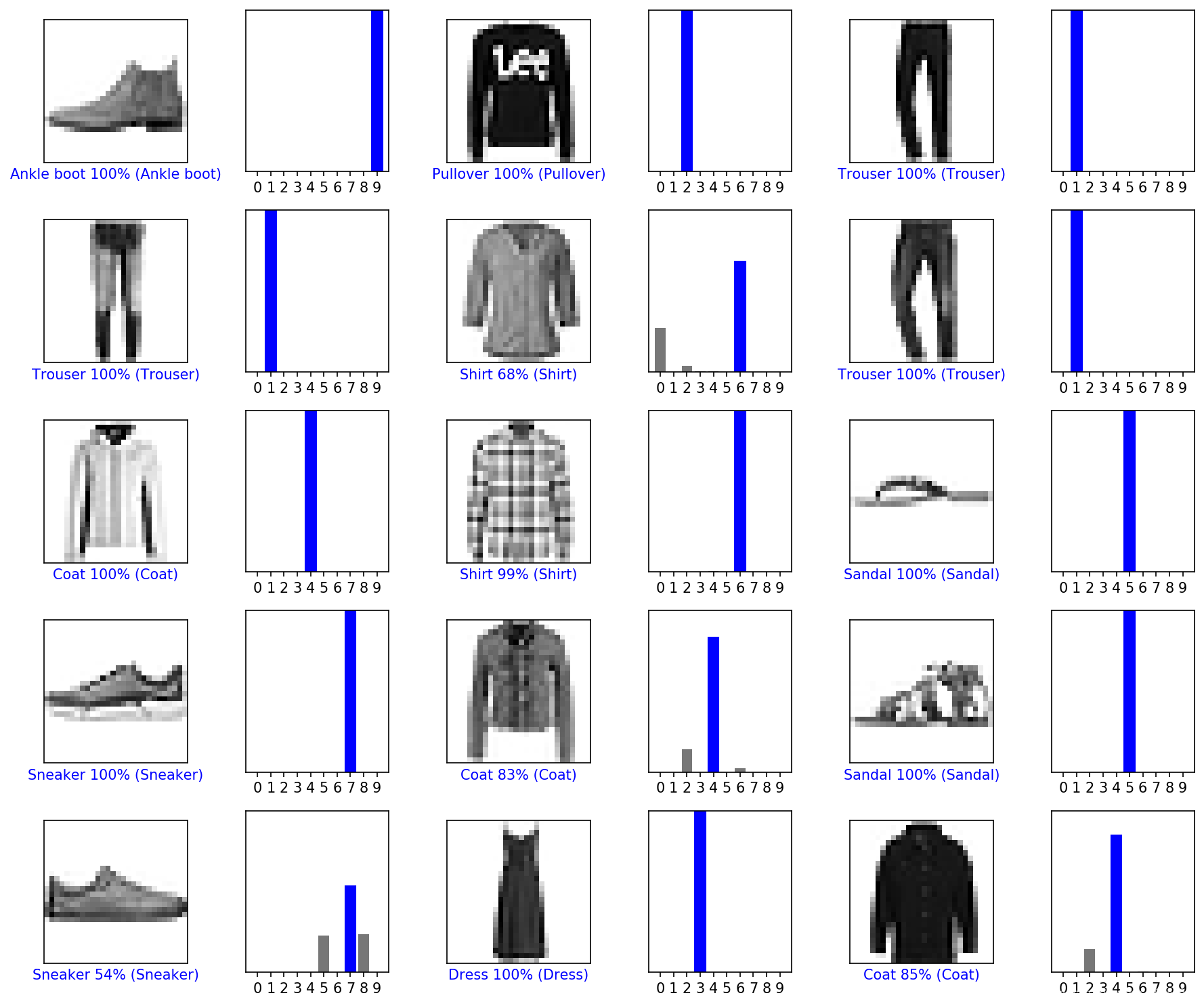
def plot_images(num_rows, num_cols):
    '''
    该函数实现多个预测结果输出
    '''
    num_images = num_rows*num_cols # 绘制图片数量
    
    plt.figure(figsize=(2*2*num_cols, 2*num_rows), dpi=150) # 设置画布尺寸
    
    for i in range(num_images):
        plt.subplot(num_rows, 2*num_cols, 2*i+1) # 第i个子图的位置
        plot_image(i, predictions[i], test_labels, test_images)
        plt.subplot(num_rows, 2*num_cols, 2*i+2)
        plot_value_array(i, predictions[i], test_labels)

    plt.tight_layout()
    plt.show()
    
   
num_rows = 5
num_cols = 3
plot_images(num_rows, num_cols)

输出：
在这里插入图片描述

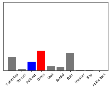
4.3 单张图片预测

def predict_image(i):
    
    img = test_images[i] # shape=(28,28)
    img = (np.expand_dims(img,0)) # shape=(1,28,28)，转化成列表格式，训练集和测试集的shape为(None,28,28)
    predictions_single = probability_model.predict(img)  # 预测
    print('predictions_single:\n', predictions_single)
    plot_value_array(1, predictions_single[0], test_labels) # 绘图
    _ = plt.xticks(range(10), class_names, rotation=45) # 设置x轴坐标刻度
    print('predict label:', np.argmax(predictions_single[0]))
    print('true label:', test_labels[i])

predict_image(66)

输出：

predictions_single:
 [[0.19836323 0.01996289 0.1276678  0.28869623 0.05913025 0.044572
  0.25288364 0.00403849 0.00407252 0.00061292]]
predict label: 3
true label: 2