Pytorch 关于nn.CrossEntropyLoss()与nn.BCEloss()以及nn.BCEWithLogitsLoss()的区别【坑】

最近用pytorch做实验，踩中一些坑，有小有大，这个问题花了我不少时间找到原因，姑且算个大坑。

首先，这几个类分别对应的函数为：

nn.CrossEntropyLoss() ——》nn.functional.cross_entropy()

nn.BCEloss() ——》nn.functional.binary_cross_entropy()

nn.BCEWithLogitsLoss() ——》nn.functional.binary_cross_entropy_with_logits()

类及其对应的函数，它们的label的形式都是一致的；同时类BCEloss()和类BCEWithLogitsLoss()的label形式是完全一致的。所以后面我直接用了函数形式，以此便于读者阅读。

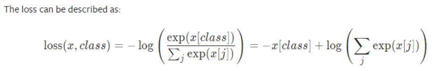
CrossEntropyLoss()是可以进行多分类的交叉熵。BCEloss()是指的二分类的交叉熵。首先在我的个人臆测中，如果做二分类的话，那既可以用CrossEntropyLoss()也可以用BCEloss()，即使输入方式不同，应该达到相同效果才对。

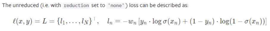
但是实际上，CrossEntropyLoss()内部将input做了softmax后再与label进行交叉熵！BCEloss()内部啥也没干直接将input与label做了交叉熵！BCEWithLogitsLoss()内部将input做了sigmoid后再与label进行交叉熵！

首先看下结果，这里没有用默认的mean，而是使用了none，也是为了读者方便观看。

input_ = torch.tensor([[0.7, 0.3]]) # 二分类，假设得到的结果为对应两个标签的概率分别为0.7,0.3，
#这里并不一定必须要加起来为1，也不一定都需要都在0-1之间，稍后解释

target1 = torch.tensor([0]) # 这里是CrossEntropy形式的label，只需要一个标签表示，假设正确标签是0（一共有0,1两种标签）
target2 = torch.tensor([[1, 0]]).to(torch.float) # 这里是BCEloss形式的label，内部是概率表示
target3 = torch.tensor([[1, 0]]).to(torch.float) # 同上，加这个target是方便读者阅读

#分别对应求loss
loss1 = torch.nn.functional.cross_entropy(input_, target1, reduction = 'none')
loss2 = torch.nn.functional.binary_cross_entropy(input_, target2, reduction = 'none')
loss3 = torch.nn.functional.binary_cross_entropy_with_logits(input_, target3, reduction = 'none')

最后的结果

loss1:
tensor([0.5130])

loss2:
tensor([[0.3567, 0.3567]])

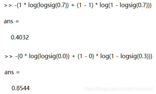
loss3:
tensor([[0.4032, 0.8544]])

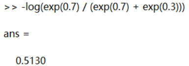
接下来验证，我用了matlab来计算

CrossEntropyLoss() / loss1

它加入了一层softmax（所以设置input并不需要加起来为1，也不一定都在0-1之间），且只对target对应的那个数进行计算，所以只有一个值：

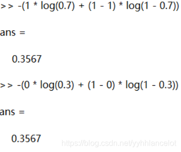
BCEloss() / loss2

它直接进行二元交叉熵计算：

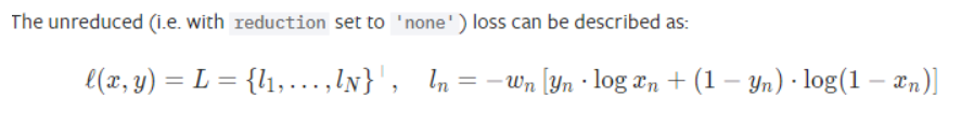
$w_n$ 是在数据不均衡时使用的，默认为1，这里忽略就好。

BCEWithLogitsLoss() / loss3

它加入了一层sigmoid，再进行二元交叉熵计算：

​

总结

博主设置input = 0.7,0.3的原因，是默认在计算loss之前经过了softmax，但没想到Pytorch好心办坏事，不过TensorFlow的开发者似乎没有Pytorch的开发者这么细致。之前觉得CrossEntropyLoss()也可以用BCEloss()在二分类应该达到相同效果才对（即softmax和sigmoid在二分类应该达到相同效果），其实是博主记混了，二分类时softmax和sigmoid确实等价

首先假设隐层输出为 $\bf h$。
如果使用sigmoid，输出层有一个节点，值为 $\bf \theta h$。
然后类别1，2的预测概率分别为

$p_1 = sigmoid(\theta h) = \frac{1}{1 +e^{-\theta h}}$

$p_2 = 1 - sigmoid(\theta h) = \frac{1}{1 +e^{\theta h}}$

如果使用softmax，则输出层有两个节点，值分别为 $\bf\theta_1 h$ 和 $\bf\theta_2 h$，然后类别1，2的预测概率为

$p_1 = \frac{e^{\theta_1 h}}{e^{\theta_1 h} +e^{\theta_2 h}} = \frac{1}{1 +e^{(\theta_2 -\theta_1) h}}$

$p_2 = \frac{e^{\theta_2 h}}{e^{\theta_1 h} +e^{\theta_2 h}} = \frac{1}{1 +e^{(\theta_1 -\theta_2) h}}$

可以看到sigmoid中的 $\bf\theta$ 是和softmax中的 $(\bf \theta_1 - \theta_2)$ 是等价的。不管sigmoid网络能产生什么样的预测，也一定存在softmax网络能产生相同的预测，只要令 $\bf \theta_1 - \theta_2 = \theta$ 就可以了。比如将0.7, 0.3输入CrossEntropyLoss()，0.4, xx输入BCEWithLogitsLoss()就会产生相同的损失值了。（xx是为了满足输入形式）。所以在纠结使用哪个loss的时候，还是看个人习惯就好，当然使用CrossEntropyLoss()更方便改用为多分类的模型。