文章目录
二手车交易价格预测 ——EDA 探索性数据分析
通过对赛题的分析,我们可以看出此类问题是对价格进行回归预测,那我们对于数据需要事先做预处理分析,这里我们采用EDA探索性数据分析来进行。
探索性数据分析是对调查,观测所得到的一些初步的杂乱无章的数据,在尽可能量少的先验假定下进行处理。通过作图,制表等形式和方程拟合计算某些特征量等手段,探索数据的结构和规律的一种数据分析方法。
对于此类问题我们可以从以下五个方面去描述分析:变量是否有缺失,变量是否有异常值,变量是否有冗余,样本是否存在不平衡问题,以及基于目标price进行分析查看各变量的分布情况。
ps:本赛题中数据链接:二手车交易数据
提取码:wqld
参考链接:https://tianchi.aliyun.com/notebook-ai/detail?spm=5176.12586969.1002.12.1cd8593aw4bbL5&postId=95457
本文基于Python3.7进行分析
1.数据的导入及数据信息的查看
import numpy as np
import pandas as pd
import warnings
import matplotlib
import matplotlib.pyplot as plt
import seaborn as sns
from scipy.special import jn
from IPython.display import display, clear_output
import time

%matplotlib inline
Train_data = pd.read_csv(r'D:\ershouche\used_car_train_20200313.csv', sep=' ')
Test_data = pd.read_csv(r'D:\ershouche\used_car_testA_20200313.csv', sep=' ')
## 2) 简略观察数据(head()+shape)
Train_data.head().append(Train_data.tail())
| SaleID | name | regDate | model | brand | bodyType | fuelType | gearbox | power | kilometer | ... | v_5 | v_6 | v_7 | v_8 | v_9 | v_10 | v_11 | v_12 | v_13 | v_14 | |
|---|---|---|---|---|---|---|---|---|---|---|---|---|---|---|---|---|---|---|---|---|---|
| 0 | 0 | 736 | 20040402 | 30.0 | 6 | 1.0 | 0.0 | 0.0 | 60 | 12.5 | ... | 0.235676 | 0.101988 | 0.129549 | 0.022816 | 0.097462 | -2.881803 | 2.804097 | -2.420821 | 0.795292 | 0.914762 |
| 1 | 1 | 2262 | 20030301 | 40.0 | 1 | 2.0 | 0.0 | 0.0 | 0 | 15.0 | ... | 0.264777 | 0.121004 | 0.135731 | 0.026597 | 0.020582 | -4.900482 | 2.096338 | -1.030483 | -1.722674 | 0.245522 |
| 2 | 2 | 14874 | 20040403 | 115.0 | 15 | 1.0 | 0.0 | 0.0 | 163 | 12.5 | ... | 0.251410 | 0.114912 | 0.165147 | 0.062173 | 0.027075 | -4.846749 | 1.803559 | 1.565330 | -0.832687 | -0.229963 |
| 3 | 3 | 71865 | 19960908 | 109.0 | 10 | 0.0 | 0.0 | 1.0 | 193 | 15.0 | ... | 0.274293 | 0.110300 | 0.121964 | 0.033395 | 0.000000 | -4.509599 | 1.285940 | -0.501868 | -2.438353 | -0.478699 |
| 4 | 4 | 111080 | 20120103 | 110.0 | 5 | 1.0 | 0.0 | 0.0 | 68 | 5.0 | ... | 0.228036 | 0.073205 | 0.091880 | 0.078819 | 0.121534 | -1.896240 | 0.910783 | 0.931110 | 2.834518 | 1.923482 |
| 149995 | 149995 | 163978 | 20000607 | 121.0 | 10 | 4.0 | 0.0 | 1.0 | 163 | 15.0 | ... | 0.280264 | 0.000310 | 0.048441 | 0.071158 | 0.019174 | 1.988114 | -2.983973 | 0.589167 | -1.304370 | -0.302592 |
| 149996 | 149996 | 184535 | 20091102 | 116.0 | 11 | 0.0 | 0.0 | 0.0 | 125 | 10.0 | ... | 0.253217 | 0.000777 | 0.084079 | 0.099681 | 0.079371 | 1.839166 | -2.774615 | 2.553994 | 0.924196 | -0.272160 |
| 149997 | 149997 | 147587 | 20101003 | 60.0 | 11 | 1.0 | 1.0 | 0.0 | 90 | 6.0 | ... | 0.233353 | 0.000705 | 0.118872 | 0.100118 | 0.097914 | 2.439812 | -1.630677 | 2.290197 | 1.891922 | 0.414931 |
| 149998 | 149998 | 45907 | 20060312 | 34.0 | 10 | 3.0 | 1.0 | 0.0 | 156 | 15.0 | ... | 0.256369 | 0.000252 | 0.081479 | 0.083558 | 0.081498 | 2.075380 | -2.633719 | 1.414937 | 0.431981 | -1.659014 |
| 149999 | 149999 | 177672 | 19990204 | 19.0 | 28 | 6.0 | 0.0 | 1.0 | 193 | 12.5 | ... | 0.284475 | 0.000000 | 0.040072 | 0.062543 | 0.025819 | 1.978453 | -3.179913 | 0.031724 | -1.483350 | -0.342674 |
10 rows × 31 columns
由此看出本次数据中包含除去saleID之外还包含30个变量,用于进行分析。
Train_data.describe()
| SaleID | name | regDate | model | brand | bodyType | fuelType | gearbox | power | kilometer | ... | v_5 | v_6 | v_7 | v_8 | v_9 | v_10 | v_11 | v_12 | v_13 | v_14 | |
|---|---|---|---|---|---|---|---|---|---|---|---|---|---|---|---|---|---|---|---|---|---|
| count | 150000.000000 | 150000.000000 | 1.500000e+05 | 149999.000000 | 150000.000000 | 145494.000000 | 141320.000000 | 144019.000000 | 150000.000000 | 150000.000000 | ... | 150000.000000 | 150000.000000 | 150000.000000 | 150000.000000 | 150000.000000 | 150000.000000 | 150000.000000 | 150000.000000 | 150000.000000 | 150000.000000 |
| mean | 74999.500000 | 68349.172873 | 2.003417e+07 | 47.129021 | 8.052733 | 1.792369 | 0.375842 | 0.224943 | 119.316547 | 12.597160 | ... | 0.248204 | 0.044923 | 0.124692 | 0.058144 | 0.061996 | -0.001000 | 0.009035 | 0.004813 | 0.000313 | -0.000688 |
| std | 43301.414527 | 61103.875095 | 5.364988e+04 | 49.536040 | 7.864956 | 1.760640 | 0.548677 | 0.417546 | 177.168419 | 3.919576 | ... | 0.045804 | 0.051743 | 0.201410 | 0.029186 | 0.035692 | 3.772386 | 3.286071 | 2.517478 | 1.288988 | 1.038685 |
| min | 0.000000 | 0.000000 | 1.991000e+07 | 0.000000 | 0.000000 | 0.000000 | 0.000000 | 0.000000 | 0.000000 | 0.500000 | ... | 0.000000 | 0.000000 | 0.000000 | 0.000000 | 0.000000 | -9.168192 | -5.558207 | -9.639552 | -4.153899 | -6.546556 |
| 25% | 37499.750000 | 11156.000000 | 1.999091e+07 | 10.000000 | 1.000000 | 0.000000 | 0.000000 | 0.000000 | 75.000000 | 12.500000 | ... | 0.243615 | 0.000038 | 0.062474 | 0.035334 | 0.033930 | -3.722303 | -1.951543 | -1.871846 | -1.057789 | -0.437034 |
| 50% | 74999.500000 | 51638.000000 | 2.003091e+07 | 30.000000 | 6.000000 | 1.000000 | 0.000000 | 0.000000 | 110.000000 | 15.000000 | ... | 0.257798 | 0.000812 | 0.095866 | 0.057014 | 0.058484 | 1.624076 | -0.358053 | -0.130753 | -0.036245 | 0.141246 |
| 75% | 112499.250000 | 118841.250000 | 2.007111e+07 | 66.000000 | 13.000000 | 3.000000 | 1.000000 | 0.000000 | 150.000000 | 15.000000 | ... | 0.265297 | 0.102009 | 0.125243 | 0.079382 | 0.087491 | 2.844357 | 1.255022 | 1.776933 | 0.942813 | 0.680378 |
| max | 149999.000000 | 196812.000000 | 2.015121e+07 | 247.000000 | 39.000000 | 7.000000 | 6.000000 | 1.000000 | 19312.000000 | 15.000000 | ... | 0.291838 | 0.151420 | 1.404936 | 0.160791 | 0.222787 | 12.357011 | 18.819042 | 13.847792 | 11.147669 | 8.658418 |
8 rows × 30 columns
## 2) 通过info()来熟悉数据类型
Train_data.info()
<class 'pandas.core.frame.DataFrame'>
RangeIndex: 150000 entries, 0 to 149999
Data columns (total 31 columns):
SaleID               150000 non-null int64
name                 150000 non-null int64
regDate              150000 non-null int64
model                149999 non-null float64
brand                150000 non-null int64
bodyType             145494 non-null float64
fuelType             141320 non-null float64
gearbox              144019 non-null float64
power                150000 non-null int64
kilometer            150000 non-null float64
notRepairedDamage    150000 non-null object
regionCode           150000 non-null int64
seller               150000 non-null int64
offerType            150000 non-null int64
creatDate            150000 non-null int64
price                150000 non-null int64
v_0                  150000 non-null float64
v_1                  150000 non-null float64
v_2                  150000 non-null float64
v_3                  150000 non-null float64
v_4                  150000 non-null float64
v_5                  150000 non-null float64
v_6                  150000 non-null float64
v_7                  150000 non-null float64
v_8                  150000 non-null float64
v_9                  150000 non-null float64
v_10                 150000 non-null float64
v_11                 150000 non-null float64
v_12                 150000 non-null float64
v_13                 150000 non-null float64
v_14                 150000 non-null float64
dtypes: float64(20), int64(10), object(1)
memory usage: 35.5+ MB
Test_data.info()
<class 'pandas.core.frame.DataFrame'>
RangeIndex: 50000 entries, 0 to 49999
Data columns (total 30 columns):
SaleID               50000 non-null int64
name                 50000 non-null int64
regDate              50000 non-null int64
model                50000 non-null float64
brand                50000 non-null int64
bodyType             48587 non-null float64
fuelType             47107 non-null float64
gearbox              48090 non-null float64
power                50000 non-null int64
kilometer            50000 non-null float64
notRepairedDamage    50000 non-null object
regionCode           50000 non-null int64
seller               50000 non-null int64
offerType            50000 non-null int64
creatDate            50000 non-null int64
v_0                  50000 non-null float64
v_1                  50000 non-null float64
v_2                  50000 non-null float64
v_3                  50000 non-null float64
v_4                  50000 non-null float64
v_5                  50000 non-null float64
v_6                  50000 non-null float64
v_7                  50000 non-null float64
v_8                  50000 non-null float64
v_9                  50000 non-null float64
v_10                 50000 non-null float64
v_11                 50000 non-null float64
v_12                 50000 non-null float64
v_13                 50000 non-null float64
v_14                 50000 non-null float64
dtypes: float64(20), int64(9), object(1)
memory usage: 11.4+ MB
通过对数据类型的查看,我们可以得到除了notRepairedDamage 的数据类型为object之外,其余都为数值型数据,但对于notRepairedDamage而言根据以上查看数据信息,可知,其实际应该为数值型数据,所以我们猜测在notRepairedDamage中包含异常值。
2.变量是否有异常值
#由上述对数据类型的分析,我们对notRepairedDamage进行检查
Train_data['notRepairedDamage'].value_counts()
0.0    111361
-       24324
1.0     14315
Name: notRepairedDamage, dtype: int64
由此可见,在notRepairedDamage中 0 有修复损坏的有111361个,1 没有修复损坏的有14315个,而缺失数据有24324个,缺失值较多,对于缺失值较多的情况,我们做删除处理
Train_data['notRepairedDamage'].replace('-', np.nan, inplace=True)
Train_data['notRepairedDamage'].value_counts()
0.0    111361
1.0     14315
Name: notRepairedDamage, dtype: int64
通过以上处理,在训练集中我们将notRepairedDamage中的空缺值删除掉了,因此此时对于变量notRepairedDamage其含有缺失值,在notRepairedDamage中 0 有修复损坏的有111361个,1 没有修复损坏的有14315个
Test_data['notRepairedDamage'].replace('-', np.nan, inplace=True)
Test_data['notRepairedDamage'].value_counts()
0.0    37249
1.0     4720
Name: notRepairedDamage, dtype: int64
同理,在训练集中我们将notRepairedDamage中的空缺值删除掉了,因此此时对于变量notRepairedDamage其含有缺失值,在notRepairedDamage中 0 有修复损坏的有37249个,1 没有修复损坏的有4720个
3.变量是否含有缺失值
Train_data.isnull().sum()
SaleID                   0
name                     0
regDate                  0
model                    1
brand                    0
bodyType              4506
fuelType              8680
gearbox               5981
power                    0
kilometer                0
notRepairedDamage    24324
regionCode               0
seller                   0
offerType                0
creatDate                0
price                    0
v_0                      0
v_1                      0
v_2                      0
v_3                      0
v_4                      0
v_5                      0
v_6                      0
v_7                      0
v_8                      0
v_9                      0
v_10                     0
v_11                     0
v_12                     0
v_13                     0
v_14                     0
dtype: int64
由此可以看出缺失数据有四类,其中在测试集中bodyType 缺失数为4506 ,fuelType 缺失数为8680;gearbox 缺失数为5981,notRepairedDamage 有24324 种
# nan可视化
missing = Train_data.isnull().sum()
missing = missing[missing > 0]
missing.sort_values(inplace=True)
missing.plot.bar()
<matplotlib.axes._subplots.AxesSubplot at 0x9cef3c8>

#查看测试集中的缺失数据
Test_data.isnull().sum()
SaleID                  0
name                    0
regDate                 0
model                   0
brand                   0
bodyType             1413
fuelType             2893
gearbox              1910
power                   0
kilometer               0
notRepairedDamage    8031
regionCode              0
seller                  0
offerType               0
creatDate               0
v_0                     0
v_1                     0
v_2                     0
v_3                     0
v_4                     0
v_5                     0
v_6                     0
v_7                     0
v_8                     0
v_9                     0
v_10                    0
v_11                    0
v_12                    0
v_13                    0
v_14                    0
dtype: int64
# nan可视化
missing = Test_data.isnull().sum()
missing = missing[missing > 0]
missing.sort_values(inplace=True)
missing.plot.bar()
<matplotlib.axes._subplots.AxesSubplot at 0x9ff42e8>

[外链图片转存失败,源站可能有防盗链机制,建议将图片保存下来直接上传(img-6adaJrRK-1585029946274)(output_22_1.png)]
总结:通过上述处理,我们可以发现具有缺失数据的变量包含四种,且对于notRepairedDamage其缺失数据最多,其他三种相对较少
而在数据处理过程中我们对弈缺失值存在的过多、可以考虑删掉,如果很小一般选择填充,如果使用lgb等树模型可以直接空缺,让树自己去优化。
4.样本是否存在不平衡问题
对于此类分析,我们可以采取逐一例举查看的方式,但此类比较麻烦,但通过我们上述,对数据的信息的查看head(),以及describe()内容,可以发现,在30个变量中‘seller’‘gearbox’,‘offerType’ 的均值,标准差等数字特征存在问题,所以我们对一下样本进行检测
Train_data['gearbox'].value_counts()
0.0    111623
1.0     32396
Name: gearbox, dtype: int64
Train_data["seller"].value_counts()
0    149999
1         1
Name: seller, dtype: int64
Train_data["offerType"].value_counts()
0    150000
Name: offerType, dtype: int64
通过检测,可以看出seller和offerType有严重的偏斜,而对于这两项可以我们可以做删除处理
#对偏斜类做删除处理
del Train_data["seller"]
del Train_data["offerType"]
del Test_data["seller"]
del Test_data["offerType"]
Train_data.describe()
| SaleID | name | regDate | model | brand | bodyType | fuelType | gearbox | power | kilometer | ... | v_5 | v_6 | v_7 | v_8 | v_9 | v_10 | v_11 | v_12 | v_13 | v_14 | |
|---|---|---|---|---|---|---|---|---|---|---|---|---|---|---|---|---|---|---|---|---|---|
| count | 150000.000000 | 150000.000000 | 1.500000e+05 | 149999.000000 | 150000.000000 | 145494.000000 | 141320.000000 | 144019.000000 | 150000.000000 | 150000.000000 | ... | 150000.000000 | 150000.000000 | 150000.000000 | 150000.000000 | 150000.000000 | 150000.000000 | 150000.000000 | 150000.000000 | 150000.000000 | 150000.000000 |
| mean | 74999.500000 | 68349.172873 | 2.003417e+07 | 47.129021 | 8.052733 | 1.792369 | 0.375842 | 0.224943 | 119.316547 | 12.597160 | ... | 0.248204 | 0.044923 | 0.124692 | 0.058144 | 0.061996 | -0.001000 | 0.009035 | 0.004813 | 0.000313 | -0.000688 |
| std | 43301.414527 | 61103.875095 | 5.364988e+04 | 49.536040 | 7.864956 | 1.760640 | 0.548677 | 0.417546 | 177.168419 | 3.919576 | ... | 0.045804 | 0.051743 | 0.201410 | 0.029186 | 0.035692 | 3.772386 | 3.286071 | 2.517478 | 1.288988 | 1.038685 |
| min | 0.000000 | 0.000000 | 1.991000e+07 | 0.000000 | 0.000000 | 0.000000 | 0.000000 | 0.000000 | 0.000000 | 0.500000 | ... | 0.000000 | 0.000000 | 0.000000 | 0.000000 | 0.000000 | -9.168192 | -5.558207 | -9.639552 | -4.153899 | -6.546556 |
| 25% | 37499.750000 | 11156.000000 | 1.999091e+07 | 10.000000 | 1.000000 | 0.000000 | 0.000000 | 0.000000 | 75.000000 | 12.500000 | ... | 0.243615 | 0.000038 | 0.062474 | 0.035334 | 0.033930 | -3.722303 | -1.951543 | -1.871846 | -1.057789 | -0.437034 |
| 50% | 74999.500000 | 51638.000000 | 2.003091e+07 | 30.000000 | 6.000000 | 1.000000 | 0.000000 | 0.000000 | 110.000000 | 15.000000 | ... | 0.257798 | 0.000812 | 0.095866 | 0.057014 | 0.058484 | 1.624076 | -0.358053 | -0.130753 | -0.036245 | 0.141246 |
| 75% | 112499.250000 | 118841.250000 | 2.007111e+07 | 66.000000 | 13.000000 | 3.000000 | 1.000000 | 0.000000 | 150.000000 | 15.000000 | ... | 0.265297 | 0.102009 | 0.125243 | 0.079382 | 0.087491 | 2.844357 | 1.255022 | 1.776933 | 0.942813 | 0.680378 |
| max | 149999.000000 | 196812.000000 | 2.015121e+07 | 247.000000 | 39.000000 | 7.000000 | 6.000000 | 1.000000 | 19312.000000 | 15.000000 | ... | 0.291838 | 0.151420 | 1.404936 | 0.160791 | 0.222787 | 12.357011 | 18.819042 | 13.847792 | 11.147669 | 8.658418 |
8 rows × 28 columns
Train_data.head()
| SaleID | name | regDate | model | brand | bodyType | fuelType | gearbox | power | kilometer | ... | v_5 | v_6 | v_7 | v_8 | v_9 | v_10 | v_11 | v_12 | v_13 | v_14 | |
|---|---|---|---|---|---|---|---|---|---|---|---|---|---|---|---|---|---|---|---|---|---|
| 0 | 0 | 736 | 20040402 | 30.0 | 6 | 1.0 | 0.0 | 0.0 | 60 | 12.5 | ... | 0.235676 | 0.101988 | 0.129549 | 0.022816 | 0.097462 | -2.881803 | 2.804097 | -2.420821 | 0.795292 | 0.914762 |
| 1 | 1 | 2262 | 20030301 | 40.0 | 1 | 2.0 | 0.0 | 0.0 | 0 | 15.0 | ... | 0.264777 | 0.121004 | 0.135731 | 0.026597 | 0.020582 | -4.900482 | 2.096338 | -1.030483 | -1.722674 | 0.245522 |
| 2 | 2 | 14874 | 20040403 | 115.0 | 15 | 1.0 | 0.0 | 0.0 | 163 | 12.5 | ... | 0.251410 | 0.114912 | 0.165147 | 0.062173 | 0.027075 | -4.846749 | 1.803559 | 1.565330 | -0.832687 | -0.229963 |
| 3 | 3 | 71865 | 19960908 | 109.0 | 10 | 0.0 | 0.0 | 1.0 | 193 | 15.0 | ... | 0.274293 | 0.110300 | 0.121964 | 0.033395 | 0.000000 | -4.509599 | 1.285940 | -0.501868 | -2.438353 | -0.478699 |
| 4 | 4 | 111080 | 20120103 | 110.0 | 5 | 1.0 | 0.0 | 0.0 | 68 | 5.0 | ... | 0.228036 | 0.073205 | 0.091880 | 0.078819 | 0.121534 | -1.896240 | 0.910783 | 0.931110 | 2.834518 | 1.923482 |
5 rows × 29 columns
现在通过所得到的5*19的表我们可以发现已经将“seller”,“offerType”,变量已经删除,以及剩余数据的数字特征信息。
5.变量之间是否存在冗余
在普通回归模型进行预测时,我们一般要考虑各变量间是否存在多重共线性,即变量间是否存在冗余的情况,此时我们可以通过查看各变量之间的相关系数r,或者决定系数R^2来判断,其是否存在多重共线性。可以尝试看变量间的R平方是不是很接近1,越接近1,说明多重共线性越明显。
当然在XGB和随机森林等模型中不需要考虑。
另外我们通过对以上各变量的查看分析,可以将变量分类,分为数字和类别两类。我们由此重点查看数字变量之间的多重共线性情况。
Y_trian=Train_data['price']
# 这个区别方式适用于没有直接label coding的数据
# 这里不适用,需要人为根据实际含义来区分
# 数字特征
#########numeric_features = Train_data.select_dtypes(include=[np.number])
######numeric_features.columns
# # 类型特征
####categorical_features = Train_data.select_dtypes(include=[np.object])
####categorical_features.columns
#人为根据实际含义来区分数字和类别nts
number=['power','kilometer','v_0','v_1','v_2','v_3','v_4','v_5','v_6','v_7','v_8','v_9','v_10','v_11','v_12','v_13','v_14']
categorical=['name','model','brand','bodyType','fuelType','gearbox','regionCode']
下面我们查看number组中各变量之间的相关系数来判断各变量之间的多重共线性,我们以0.9作为阈值判断,若大于0.9,则判断其存在多重共线性
#相关性分析
price_number=Train_data[number]
corr=price_number.corr()
corr
| power | kilometer | v_0 | v_1 | v_2 | v_3 | v_4 | v_5 | v_6 | v_7 | v_8 | v_9 | v_10 | v_11 | v_12 | v_13 | v_14 | |
|---|---|---|---|---|---|---|---|---|---|---|---|---|---|---|---|---|---|
| power | 1.000000 | -0.019631 | 0.215028 | 0.023746 | -0.031487 | -0.185342 | -0.141013 | 0.119727 | 0.025648 | -0.060397 | 0.155956 | -0.140203 | -0.092717 | -0.122107 | 0.161990 | -0.103430 | -0.023808 |
| kilometer | -0.019631 | 1.000000 | -0.225034 | -0.022228 | -0.110375 | 0.402502 | -0.214861 | 0.049502 | -0.024664 | -0.017835 | -0.407686 | -0.149422 | 0.083358 | 0.066542 | -0.370153 | -0.285158 | -0.120389 |
| v_0 | 0.215028 | -0.225034 | 1.000000 | 0.245049 | -0.452591 | -0.710480 | -0.259714 | 0.726250 | 0.243783 | -0.584363 | 0.514149 | -0.186243 | -0.582943 | -0.667809 | 0.415711 | -0.136938 | -0.039809 |
| v_1 | 0.023746 | -0.022228 | 0.245049 | 1.000000 | -0.001133 | -0.001915 | -0.000468 | 0.109303 | 0.999415 | -0.110806 | -0.298966 | -0.007698 | -0.921904 | 0.370445 | -0.087593 | 0.017349 | 0.002143 |
| v_2 | -0.031487 | -0.110375 | -0.452591 | -0.001133 | 1.000000 | 0.001224 | -0.001021 | -0.921857 | 0.023877 | 0.973689 | 0.180285 | -0.236164 | 0.274341 | 0.800915 | 0.535270 | -0.055376 | -0.013785 |
| v_3 | -0.185342 | 0.402502 | -0.710480 | -0.001915 | 0.001224 | 1.000000 | -0.001694 | -0.233412 | -0.000747 | 0.191278 | -0.933161 | 0.079292 | 0.247385 | 0.429777 | -0.811301 | -0.246052 | -0.058561 |
| v_4 | -0.141013 | -0.214861 | -0.259714 | -0.000468 | -0.001021 | -0.001694 | 1.000000 | -0.259739 | -0.011275 | -0.054241 | 0.051741 | 0.962928 | 0.071116 | 0.110660 | -0.134611 | 0.934580 | -0.178518 |
| v_5 | 0.119727 | 0.049502 | 0.726250 | 0.109303 | -0.921857 | -0.233412 | -0.259739 | 1.000000 | 0.091229 | -0.939385 | 0.010686 | -0.050343 | -0.440588 | -0.845954 | -0.258521 | -0.162689 | 0.037804 |
| v_6 | 0.025648 | -0.024664 | 0.243783 | 0.999415 | 0.023877 | -0.000747 | -0.011275 | 0.091229 | 1.000000 | -0.085410 | -0.294956 | -0.023057 | -0.917056 | 0.386446 | -0.070238 | 0.000758 | -0.003322 |
| v_7 | -0.060397 | -0.017835 | -0.584363 | -0.110806 | 0.973689 | 0.191278 | -0.054241 | -0.939385 | -0.085410 | 1.000000 | 0.028695 | -0.264091 | 0.410014 | 0.813175 | 0.385378 | -0.154535 | -0.020218 |
| v_8 | 0.155956 | -0.407686 | 0.514149 | -0.298966 | 0.180285 | -0.933161 | 0.051741 | 0.010686 | -0.294956 | 0.028695 | 1.000000 | -0.063577 | 0.094497 | -0.369353 | 0.882121 | 0.250423 | 0.030416 |
| v_9 | -0.140203 | -0.149422 | -0.186243 | -0.007698 | -0.236164 | 0.079292 | 0.962928 | -0.050343 | -0.023057 | -0.264091 | -0.063577 | 1.000000 | 0.026562 | -0.056200 | -0.313634 | 0.880545 | -0.214151 |
| v_10 | -0.092717 | 0.083358 | -0.582943 | -0.921904 | 0.274341 | 0.247385 | 0.071116 | -0.440588 | -0.917056 | 0.410014 | 0.094497 | 0.026562 | 1.000000 | 0.006306 | 0.001289 | -0.000580 | 0.002244 |
| v_11 | -0.122107 | 0.066542 | -0.667809 | 0.370445 | 0.800915 | 0.429777 | 0.110660 | -0.845954 | 0.386446 | 0.813175 | -0.369353 | -0.056200 | 0.006306 | 1.000000 | 0.006695 | -0.001671 | -0.001156 |
| v_12 | 0.161990 | -0.370153 | 0.415711 | -0.087593 | 0.535270 | -0.811301 | -0.134611 | -0.258521 | -0.070238 | 0.385378 | 0.882121 | -0.313634 | 0.001289 | 0.006695 | 1.000000 | 0.001512 | 0.002045 |
| v_13 | -0.103430 | -0.285158 | -0.136938 | 0.017349 | -0.055376 | -0.246052 | 0.934580 | -0.162689 | 0.000758 | -0.154535 | 0.250423 | 0.880545 | -0.000580 | -0.001671 | 0.001512 | 1.000000 | 0.001419 |
| v_14 | -0.023808 | -0.120389 | -0.039809 | 0.002143 | -0.013785 | -0.058561 | -0.178518 | 0.037804 | -0.003322 | -0.020218 | 0.030416 | -0.214151 | 0.002244 | -0.001156 | 0.002045 | 0.001419 | 1.000000 |
f , ax = plt.subplots(figsize = (7, 7))

plt.title('Correlation of Numeric Features with Price',y=1,size=16)

sns.heatmap(corr,square = True,  vmax=0.8)
<matplotlib.axes._subplots.AxesSubplot at 0xa3b8048>

通过对以上的相关性分析,我们可以看出存在五组变量的相关系数>0.9, 其分别为corr(v_7,v_2)=0.973689,corr(v_7,v_5)=0.939385,corr(v_8,v_3)=0.933161,corr(v_13,v_4)=0.93580,corr(v_1,v_6)=0.999416
由此,对于存在多重共线性的变量,我们可以采取删除的方式处理。
下面我们我们先查看各变量的分布特征,以及其对目标price的影响,再来判断应该删除的变量。
6.基于目标price进行分析查看各变量的分布情况
Train_data['price']
0          1850
1          3600
2          6222
3          2400
4          5200
5          8000
6          3500
7          1000
8          2850
9           650
10         3100
11         5450
12         1600
13         3100
14         6900
15         3200
16        10500
17         3700
18          790
19         1450
20          990
21         2800
22          350
23          599
24         9250
25         3650
26         2800
27         2399
28         4900
29         2999
          ...
149970      900
149971     3400
149972      999
149973     3500
149974     4500
149975     3990
149976     1200
149977      330
149978     3350
149979     5000
149980     4350
149981     9000
149982     2000
149983    12000
149984     6700
149985     4200
149986     2800
149987     3000
149988     7500
149989     1150
149990      450
149991    24950
149992      950
149993     4399
149994    14780
149995     5900
149996     9500
149997     7500
149998     4999
149999     4700
Name: price, Length: 150000, dtype: int64
import scipy.stats as st
y = Train_data['price']
plt.figure(1); plt.title('Johnson SU')  #无界约翰逊分布
sns.distplot(y, kde=False, fit=st.johnsonsu)
plt.figure(2); plt.title('Normal')
sns.distplot(y, kde=False, fit=st.norm)
plt.figure(3); plt.title('Log Normal')
sns.distplot(y, kde=False, fit=st.lognorm)


Train_data.columns
Index(['SaleID', 'name', 'regDate', 'model', 'brand', 'bodyType', 'fuelType',
       'gearbox', 'power', 'kilometer', 'notRepairedDamage', 'regionCode',
       'creatDate', 'price', 'v_0', 'v_1', 'v_2', 'v_3', 'v_4', 'v_5', 'v_6',
       'v_7', 'v_8', 'v_9', 'v_10', 'v_11', 'v_12', 'v_13', 'v_14'],
      dtype='object')
价格不服从正态分布,所以在进行回归之前,它必须进行转换。虽然对数变换做得很好,但最佳拟合是无界约翰逊分布 约翰逊分布体系可以将非正态转为正态可以参考约翰逊分布体系,
然后因为非正态,可以看一下其峰度和偏度。
#查看其skewness  and  kurtosis
sns.distplot(Train_data['price']);
print("Skewness: %f" % Train_data['price'].skew())
print("Kurtosis: %f" % Train_data['price'].kurt())
Skewness: 3.346487
Kurtosis: 18.995183
由此可看出其偏度值为3.346487,而其峰度为18.9958183,可以看出其为非正态分布
## 3) 查看预测值的具体频数
plt.hist(Train_data['price'], orientation = 'vertical',histtype = 'bar', color ='red')
plt.show()

通过查看频数分布,我们可以看出,大部分的交易价格在0-20000的区间内。我们对其进行log变换,看其稍微更具体的均匀分布
plt.hist(np.log(Train_data['price']), orientation = 'vertical',histtype = 'bar', color ='red')
plt.show()

由此可以看到大部分的交易价格在10000左右。
在变量是否存在冗余部分我们对数据进行的分类,接下来我们从分类变量和数值变量两个方面,查看分析其对目标变量price的影响
6.1类别变量对price的影响分析
#类别特征分布
for cat in categorical:
    print(cat+ "特征分布:")
    print("{}特征有{}个不同的值".format(cat,Train_data[cat].nunique()))
    print(Train_data[cat].value_counts())
name特征分布:
name特征有99662个不同的值
708       282
387       282
55        280
1541      263
203       233
53        221
713       217
290       197
1186      184
911       182
2044      176
1513      160
1180      158
631       157
893       153
2765      147
473       141
1139      137
1108      132
444       129
306       127
2866      123
2402      116
533       114
1479      113
422       113
4635      110
725       110
964       109
1373      104
         ...
89083       1
95230       1
164864      1
173060      1
179207      1
181256      1
185354      1
25564       1
19417       1
189324      1
162719      1
191373      1
193422      1
136082      1
140180      1
144278      1
146327      1
148376      1
158621      1
1404        1
15319       1
46022       1
64463       1
976         1
3025        1
5074        1
7123        1
11221       1
13270       1
174485      1
Name: name, Length: 99662, dtype: int64
model特征分布:
model特征有248个不同的值
0.0      11762
19.0      9573
4.0       8445
1.0       6038
29.0      5186
48.0      5052
40.0      4502
26.0      4496
8.0       4391
31.0      3827
13.0      3762
17.0      3121
65.0      2730
49.0      2608
46.0      2454
30.0      2342
44.0      2195
5.0       2063
10.0      2004
21.0      1872
73.0      1789
11.0      1775
23.0      1696
22.0      1524
69.0      1522
63.0      1469
7.0       1460
16.0      1349
88.0      1309
66.0      1250
         ...
141.0       37
133.0       35
216.0       30
202.0       28
151.0       26
226.0       26
231.0       23
234.0       23
233.0       20
198.0       18
224.0       18
227.0       17
237.0       17
220.0       16
230.0       16
239.0       14
223.0       13
236.0       11
241.0       10
232.0       10
229.0       10
235.0        7
246.0        7
243.0        4
244.0        3
245.0        2
209.0        2
240.0        2
242.0        2
247.0        1
Name: model, Length: 248, dtype: int64
brand特征分布:
brand特征有40个不同的值
0     31480
4     16737
14    16089
10    14249
1     13794
6     10217
9      7306
5      4665
13     3817
11     2945
3      2461
7      2361
16     2223
8      2077
25     2064
27     2053
21     1547
15     1458
19     1388
20     1236
12     1109
22     1085
26      966
30      940
17      913
24      772
28      649
32      592
29      406
37      333
2       321
31      318
18      316
36      228
34      227
33      218
23      186
35      180
38       65
39        9
Name: brand, dtype: int64
bodyType特征分布:
bodyType特征有8个不同的值
0.0    41420
1.0    35272
2.0    30324
3.0    13491
4.0     9609
5.0     7607
6.0     6482
7.0     1289
Name: bodyType, dtype: int64
fuelType特征分布:
fuelType特征有7个不同的值
0.0    91656
1.0    46991
2.0     2212
3.0      262
4.0      118
5.0       45
6.0       36
Name: fuelType, dtype: int64
gearbox特征分布:
gearbox特征有2个不同的值
0.0    111623
1.0     32396
Name: gearbox, dtype: int64
regionCode特征分布:
regionCode特征有7905个不同的值
419     369
764     258
125     137
176     136
462     134
428     132
24      130
1184    130
122     129
828     126
70      125
827     120
207     118
1222    117
2418    117
85      116
2615    115
2222    113
759     112
188     111
1757    110
1157    109
2401    107
1069    107
3545    107
424     107
272     107
451     106
450     105
129     105
       ...
6324      1
7372      1
7500      1
8107      1
2453      1
7942      1
5135      1
6760      1
8070      1
7220      1
8041      1
8012      1
5965      1
823       1
7401      1
8106      1
5224      1
8117      1
7507      1
7989      1
6505      1
6377      1
8042      1
7763      1
7786      1
6414      1
7063      1
4239      1
5931      1
7267      1
Name: regionCode, Length: 7905, dtype: int64
#test
for cat in categorical:
    print(cat+ "特征分布:")
    print("{}特征有{}个不同的值".format(cat,Test_data[cat].nunique()))
    print(Test_data[cat].value_counts())
name特征分布:
name特征有37453个不同的值
55        97
708       96
387       95
1541      88
713       74
53        72
1186      67
203       67
631       65
911       64
2044      62
2866      60
1139      57
893       54
1180      52
2765      50
1108      50
290       48
1513      47
691       45
473       44
299       43
444       41
422       39
964       39
1479      38
1273      38
306       36
725       35
4635      35
          ..
46786      1
48835      1
165572     1
68204      1
171719     1
59080      1
186062     1
11985      1
147155     1
134869     1
138967     1
173792     1
114403     1
59098      1
59144      1
40679      1
61161      1
128746     1
55022      1
143089     1
14066      1
147187     1
112892     1
46598      1
159481     1
22270      1
89855      1
42752      1
48899      1
11808      1
Name: name, Length: 37453, dtype: int64
model特征分布:
model特征有247个不同的值
0.0      3896
19.0     3245
4.0      3007
1.0      1981
29.0     1742
48.0     1685
26.0     1525
40.0     1409
8.0      1397
31.0     1292
13.0     1210
17.0     1087
65.0      915
49.0      866
46.0      831
30.0      803
10.0      709
5.0       696
44.0      676
21.0      659
11.0      603
23.0      591
73.0      561
69.0      555
7.0       526
63.0      493
22.0      443
16.0      412
66.0      411
88.0      391
         ...
124.0       9
193.0       9
151.0       8
198.0       8
181.0       8
239.0       7
233.0       7
216.0       7
231.0       6
133.0       6
236.0       6
227.0       6
220.0       5
230.0       5
234.0       4
224.0       4
241.0       4
223.0       4
229.0       3
189.0       3
232.0       3
237.0       3
235.0       2
245.0       2
209.0       2
242.0       1
240.0       1
244.0       1
243.0       1
246.0       1
Name: model, Length: 247, dtype: int64
brand特征分布:
brand特征有40个不同的值
0     10348
4      5763
14     5314
10     4766
1      4532
6      3502
9      2423
5      1569
13     1245
11      919
7       795
3       773
16      771
8       704
25      695
27      650
21      544
15      511
20      450
19      450
12      389
22      363
30      324
17      317
26      303
24      268
28      225
32      193
29      117
31      115
18      106
2       104
37       92
34       77
33       76
36       67
23       62
35       53
38       23
39        2
Name: brand, dtype: int64
bodyType特征分布:
bodyType特征有8个不同的值
0.0    13985
1.0    11882
2.0     9900
3.0     4433
4.0     3303
5.0     2537
6.0     2116
7.0      431
Name: bodyType, dtype: int64
fuelType特征分布:
fuelType特征有7个不同的值
0.0    30656
1.0    15544
2.0      774
3.0       72
4.0       37
6.0       14
5.0       10
Name: fuelType, dtype: int64
gearbox特征分布:
gearbox特征有2个不同的值
0.0    37301
1.0    10789
Name: gearbox, dtype: int64
regionCode特征分布:
regionCode特征有6971个不同的值
419     146
764      78
188      52
125      51
759      51
2615     50
462      49
542      44
85       44
1069     43
451      41
828      40
757      39
1688     39
2154     39
1947     39
24       39
2690     38
238      38
2418     38
827      38
1184     38
272      38
233      38
70       37
703      37
2067     37
509      37
360      37
176      37
       ...
5512      1
7465      1
1290      1
3717      1
1258      1
7401      1
7920      1
7925      1
5151      1
7527      1
7689      1
8114      1
3237      1
6003      1
7335      1
3984      1
7367      1
6001      1
8021      1
3691      1
4920      1
6035      1
3333      1
5382      1
6969      1
7753      1
7463      1
7230      1
826       1
112       1
Name: regionCode, Length: 6971, dtype: int64
## 1) unique分布
for fea in categorical:
    print(Train_data[fea].nunique())
99662
248
40
8
7
2
7905
由此可以知道在categorical=[‘name’,‘model’,‘brand’,‘bodyType’,‘fuelType’,‘gearbox’,‘regionCode’]中,其分别有99662,248,40,8,7,2,7905种。
接下来分析各类别变量与目标变量之间的关系
#类别特征箱形图可视化

# 因为 name和 regionCode的类别太稀疏了,这里我们把不稀疏的几类画一下
categorical_features = ['model',
 'brand',
 'bodyType',
 'fuelType',
 'gearbox',
 'notRepairedDamage']
for c in categorical_features:
    Train_data[c] = Train_data[c].astype('category')
    if Train_data[c].isnull().any():
        Train_data[c] = Train_data[c].cat.add_categories(['MISSING'])
        Train_data[c] = Train_data[c].fillna('MISSING')

def boxplot(x, y, **kwargs):
    sns.boxplot(x=x, y=y)
    x=plt.xticks(rotation=90)

f = pd.melt(Train_data, id_vars=['price'], value_vars=categorical_features)
g = sns.FacetGrid(f, col="variable",  col_wrap=2, sharex=False, sharey=False, size=5)
g = g.map(boxplot, "value", "price")
C:\ProgramData\Anaconda3\lib\site-packages\seaborn\axisgrid.py:230: UserWarning: The `size` paramter has been renamed to `height`; please update your code.
  warnings.warn(msg, UserWarning)

通过可视化图形,我们可以观察到各类别对情况下其价格的中位数大多数都分布在10000左右,而在5000附近的分布更是居多,且其对价格都有一定的影响。
而在通过箱线图我们可以发现其均存在较多的异常值,在之后的特征工程中,我们会删除这些异常值。
## 4) 类别特征的柱形图可视化
def bar_plot(x, y, **kwargs):
    sns.barplot(x=x, y=y)
    x=plt.xticks(rotation=90)

f = pd.melt(Train_data, id_vars=['price'], value_vars=categorical_features)
g = sns.FacetGrid(f, col="variable",  col_wrap=2, sharex=False, sharey=False, size=5)
g = g.map(bar_plot, "value", "price")
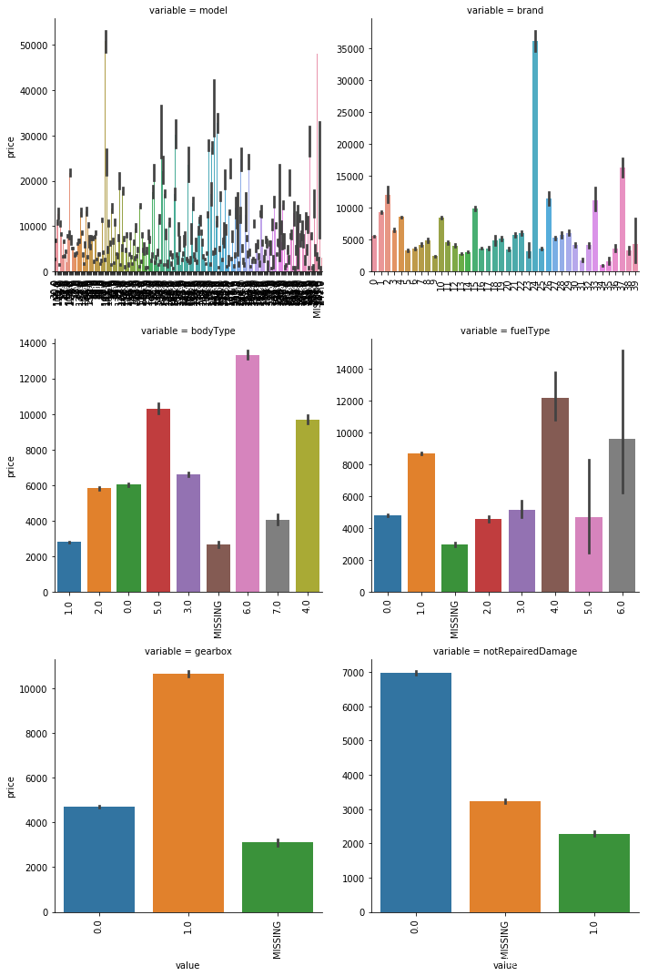
而我们类别特征柱形图可视化之后,可以更清楚的了解,各类别变量的在不太情况下其对样本的影响,对于数量brand类别我们可以看出在24点的price一枝独秀,都较为平均位于20000以下,以gearbox和notRepaireDamage来讲,其有变速箱和无修复损坏的车辆其交易价格明显更高,可以看出该变量对价格有着更为明显的影响。
6.2数值变量对price的影响分析
#查看各变量对目标变量price的相关关系
n_p = number.append('price')
#相关性分析
price_number=Train_data[number]
corr=price_number.corr()
print(corr['price'].sort_values())
v_3         -0.730946
kilometer   -0.440519
v_11        -0.275320
v_10        -0.246175
v_9         -0.206205
v_4         -0.147085
v_7         -0.053024
v_13        -0.013993
v_14         0.035911
v_1          0.060914
v_6          0.068970
v_2          0.085322
v_5          0.164317
power        0.219834
v_0          0.628397
v_8          0.685798
v_12         0.692823
price        1.000000
Name: price, dtype: float64
#可视化图象
f , ax = plt.subplots(figsize = (7, 7))

plt.title('Correlation of Numeric Features with Price',y=1,size=16)

sns.heatmap(corr,square = True,  vmax=0.8)
<matplotlib.axes._subplots.AxesSubplot at 0xa762c50>
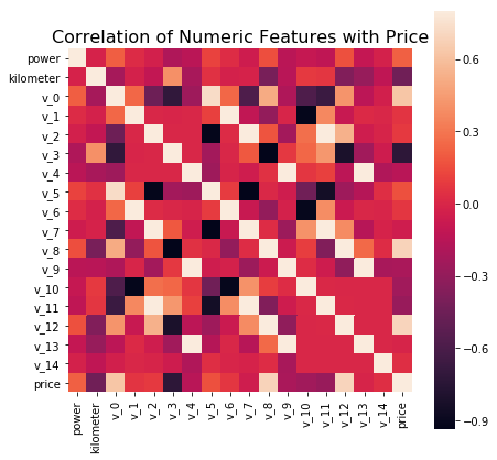
我们选取其相关系数绝对值>1的变量,进行相关分析,可知其包含变量
‘v_3’,‘v_12’,‘v_8’,‘v_0’,‘v_5’,‘v_11’,‘v_10’,‘v_9’,‘v_4’,‘power’,‘kilometor’
另,在上述数值变量之间是否存在冗余中,我们分析得到corr(v_8,v_3)=0.933161,即其存在多重共线性,所以,最终我们选取十个变量’v_3’,‘v_12’,‘v_0’,‘v_5’,‘v_11’,‘v_10’,‘v_9’,‘v_4’,‘power’,'kilometor’对目标变量price进行分析。
Y_train=Train_data['price']
Y_trian
0          1850
1          3600
2          6222
3          2400
4          5200
5          8000
6          3500
7          1000
8          2850
9           650
10         3100
11         5450
12         1600
13         3100
14         6900
15         3200
16        10500
17         3700
18          790
19         1450
20          990
21         2800
22          350
23          599
24         9250
25         3650
26         2800
27         2399
28         4900
29         2999
          ...
149970      900
149971     3400
149972      999
149973     3500
149974     4500
149975     3990
149976     1200
149977      330
149978     3350
149979     5000
149980     4350
149981     9000
149982     2000
149983    12000
149984     6700
149985     4200
149986     2800
149987     3000
149988     7500
149989     1150
149990      450
149991    24950
149992      950
149993     4399
149994    14780
149995     5900
149996     9500
149997     7500
149998     4999
149999     4700
Name: price, Length: 150000, dtype: int64
## 5) 多变量互相回归关系可视化
columns = ['price','v_3','v_12','v_0','v_5','v_11','v_10','v_9','v_4','power','kilometer']
fig, ((ax1, ax2), (ax3, ax4), (ax5, ax6), (ax7, ax8), (ax9, ax10)) = plt.subplots(nrows=5, ncols=2, figsize=(24, 20))
#[v_3','v_12','v_0','v_5','v_11','v_10','v_9','v_4','power','kilometer']
v_12_scatter_plot = pd.concat([Y_train,Train_data['v_12']],axis = 1)
sns.regplot(x='v_12',y = 'price', data = v_12_scatter_plot,scatter= True, fit_reg=True, ax=ax1)

v_3_scatter_plot = pd.concat([Y_train,Train_data['v_3']],axis = 1)
sns.regplot(x='v_3',y = 'price',data = v_3_scatter_plot,scatter= True, fit_reg=True, ax=ax2)

v_0_scatter_plot = pd.concat([Y_train,Train_data['v_0']],axis = 1)
sns.regplot(x='v_0',y = 'price',data = v_0_scatter_plot,scatter= True, fit_reg=True, ax=ax3)

power_scatter_plot = pd.concat([Y_train,Train_data['power']],axis = 1)
sns.regplot(x='power',y = 'price',data = power_scatter_plot,scatter= True, fit_reg=True, ax=ax4)

v_5_scatter_plot = pd.concat([Y_train,Train_data['v_5']],axis = 1)
sns.regplot(x='v_5',y = 'price',data = v_5_scatter_plot,scatter= True, fit_reg=True, ax=ax5)

v_11_scatter_plot = pd.concat([Y_train,Train_data['v_11']],axis = 1)
sns.regplot(x='v_11',y = 'price',data = v_11_scatter_plot,scatter= True, fit_reg=True, ax=ax6)
v_10_scatter_plot = pd.concat([Y_train,Train_data['v_10']],axis = 1)
sns.regplot(x='v_10',y = 'price',data = v_10_scatter_plot,scatter= True, fit_reg=True, ax=ax7)

v_9_scatter_plot = pd.concat([Y_train,Train_data['v_9']],axis = 1)
sns.regplot(x='v_9',y = 'price',data = v_9_scatter_plot,scatter= True, fit_reg=True, ax=ax8)

v_4_scatter_plot = pd.concat([Y_train,Train_data['v_4']],axis = 1)
sns.regplot(x='v_4',y = 'price',data = v_4_scatter_plot,scatter= True, fit_reg=True, ax=ax9)

kilometer_scatter_plot = pd.concat([Y_train,Train_data['kilometer']],axis = 1)
sns.regplot(x='kilometer',y = 'price',data = kilometer_scatter_plot,scatter= True, fit_reg=True, ax=ax10)
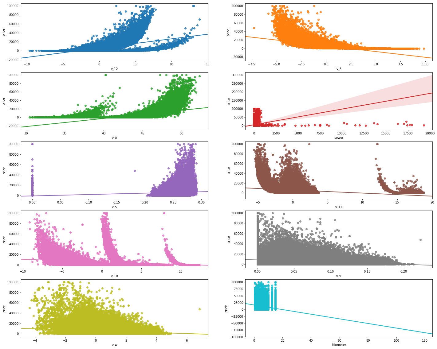
从可视化图形我们可以清晰地看出v_3,kilometer,v_11,v_10,v_9,v_4对目标变量呈现大幅度的负向影响,而v_12,v_0,v_5,power存在负向影响。
总结
通过以上分析我们对数据中的30个变量进行处理分可知:
1.存在异常值的变量为notRepaireDamage,再对其进行去non处理后,得到具有缺失值的变量有bodyType,fuelType,gearbox,notRepaireDamage,故,在后续特征工程中我们需要对此类数据进行处理
2.不平衡变量有seller,offerType,我们对其进行了删除处理
3.将变量人为化为数值变量和类别变量,变量的是否存在冗余分析过程中,得到存在强相关性的几个数值变量分别为:corr(v_7,v_2)=0.973689,corr(v_7,v_5)=0.939385,corr(v_8,v_3)=0.933161,corr(v_13,v_4)=0.93580,corr(v_1,v_6)=0.999416
4.对于数值变量与价格之间的相关程度分析,以及综合上述3所得到的存在多重共线性的数值变量,我们将选取10个最具代表性的数值变量[v_3’,‘v_12’,‘v_0’,‘v_5’,‘v_11’,‘v_10’,‘v_9’,‘v_4’,‘power’,‘kilometer’],进行之后的工作,而类别变量中我们选取不太稀疏的[‘model’, ‘brand’, ‘bodyType’, ‘fuelType’, ‘gearbox’, ‘notRepairedDamage’],进行分析。
