机器学习-P3 梯度下降法

1，介绍

基本原理

梯度下降
不是一个机器学习的算法
是一个基于搜索的最优化方法
作用：最小化一个损失函数

梯度上升法：最大化一个效用函数

（不管在最低点哪一侧都会是，都会是下降的）

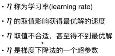
关于参数eta

并不是所有函数都有唯一的极值点

解决方法：
多次运行，随机化初始点
梯度下降法的初始值也是一个超参数

2，代码实现

会用到的库

import numpy as np
import matplotlib.pyplot as plt

原材料

首先建立一个简单的数据

# [-1,6]的等差数列，包含141个数值
plot_x = np.linspace(-1, 6, 141)

不同的算法会有不同的损失函数

# 损失函数
plot_y = (plot_x-2.5)**2-1

def J(theta):
    return (theta-2.5)**2-1

大概长成这个样子

plt.plot(plot_x,plot_y)
plt.show()

损失函数求导

def dJ(theta):
    return 2*(theta-2.5)

简单地梯度下降

eta：参数eta
epsilon：精度（不能保证刚好能取到最低点，所以当临近两次结果差值小于精度时停止）
theta_history：所有的损失值
theta：起始点

eta = 0.1
epsilon = 0.01
theta_history = [theta]
theta = 0.0
while True:
    gradient = dJ(theta)
    last_theat = theta #为了进行对比需要存储上一个损失值
    theta = theta - eta*gradient
    theta_history.append(theta)
    
    if (abs(J(theta) - J(last_theat)) < epsilon):
        break
        
print(theta)
print(J(theta))

plt.plot(plot_x,J(plot_x)) 
plt.scatter(np.array(theta_history),J(np.array(theta_history)),color='r',marker='+')
plt.show()
>>>2.499891109642585
>>>-0.99999998814289

下降了15次

len(theta_history)
>>>15

3，简单地封装一下

class Gradient_Descent:

    def __init__(self, x, y):
        self.theta_history = None
        self.x = x
        self.y = y

    # 损失函数求导
    def _dJ(theta):
        return 2 * (theta - 2.5)

    # 损失函数（根据不同算法是会变的）
    def _J(theta):
        return (theta - 2.5) ** 2 - 1

    def gradinet_descent(self,initial_theta, eta, n_iters=100, epsilon=1e-8):
        """

        :param initial_theta: 起始值
        :param eta: 每次下降的步幅
        :param n_iters: 最大下降次数，以防eta过大导致无限循环
        :param epsilon: 精度
        """
        theta = initial_theta
        self.theta_history.append(initial_theta)
        i_iters = 0

        while i_iters < n_iters:
            gradient = self._dJ(theta)
            last_theat = theta
            theta = theta - eta * gradient
            self.theta_history.append(theta)
            if abs(self._J(theta) - self._J(last_theat)) < epsilon:
                break
            i_iters += 1

    def plot_theta_history(self):
        """
        观察下降走势
        :return:
        """
        plt.plot(self.x, self._J(self.x))
        plt.plot(np.array(self.theta_history), self._J(np.array(self.theta_history)), color='r', marker='+')
        plt.show()

关于参数

eta的大小对回归的影响
1，当eta很小时，下降步幅会很小，从而我们的得到的theta_history会更大

eta = 0.01
theta_history = []
gradinet_descent(0.,eta)
plot_theta_history()

len(theta_history)
>>>424

2，当eta大的合理时，会发现他不一定只从单边下降，会跳点的

eta = 0.8
theta_history = []
gradinet_descent(0.,eta)
plot_theta_history()

3，当eta大的离谱时，函数就会报错

eta = 1.1
theta_history = []
gradinet_descent(0.,eta)
plot_theta_history()

>>>OverflowError: (34, 'Result too large')

我们也就需要有n_iters来限定下降次数

eta = 1.1
theta_history = []
gradinet_descent(0.,eta,n_iters=100)
plot_theta_history()

所以，当eta过大时，也会有可能是越来越大的，如上图（就很离谱）
当然，也刚好可能很巧和x轴平行（我就不尝试了，8年老本实在太慢）

4，多元线性回归中的梯度下降法

公式理解

即使在一元线性回归中sta都会有两个值【sta0=1，sta1】
再对每一项进行偏微分

举个例子，这是一个等高线的梯度下降法是意图
其中z为损失函数ste集包含[x, y]

得出多元线性回归的损失函数

再计算出每一项的梯度值（计算每一项偏导数）
通过公式可以看出来，每一项的大小和样本数量m有关，当m越大时，梯度值也会随之变大（就很离谱）
并不是所有的损失函数都可以直接用来进行梯度下降，有时需要特殊化

所以在下边会使用下列的J（sta）来计算梯度值

代码实现

首先需要有基本数据（先不用sklearn中的数据）

x：随机浮点数，浮点数范围 : (0,1)，共100个
y：100个正态分布[normal]的数值

x = 2 * np.random.random(size=100).reshape(-1,1)
y = x * 3. + 4. + np.random.normal(size=100)

x.shape
>>>(100, 1)
y.shape
>>>(100, )

plt.scatter(x,y)
plt.show()

根据公式得到损失函数及其导数函数
theta：
x_b：
y：真值

def J(theta, x_b, y):
    try:
        return np.sum((y - x_b.dot(theta))**2) / len(x_b)
    except:
        return float('inf')

def dJ(theta, x_b, y):
    res = np.empty(len(theta))
    res[0] = np.sum(x_b.dot(theta) - y)
    for i in range(1,len(theta)):
        res[i] = (x_b.dot(theta) - y).dot(x_b[:,i])
    return res * 2 / len(x_b)

np.empty(shape,[ dtype, order])
依据给定形状和类型(shape,[dtype, order])返回一个新的空数组。

def gradinet_descent(x_b, y, initial_theta, eta, n_iters = 100, epsilon=1e-8):
    
    theta = initial_theta
    i_iters = 0
    
    while i_iters < n_iters:
        gradient = dJ(theta, x_b, y)
        last_theat = theta
        theta = theta - eta * gradient

        if (abs(J(theta, x_b, y) - J(last_theat, x_b, y)) < epsilon):
            break
            
        i_iters += 1
        
    return theta

看一下效果

x_b = np.hstack([np.ones((len(x), 1)) ,x.reshape(-1,1)])
initial_theta = np.zeros(x_b.shape[1])
eta = 0.01

gradinet_descent(x_b, y, initial_theta, eta)
>>>array([3.21783895, 3.52422368])

使用向量化计算进行封装

先看一下公式吧（不管看得懂看不懂的）

这边我直接把它加在线性回归函数里了
方法：fit_gd（）

import numpy as np


class LinearRegression:

    def __init__(self):
        self.coef_ = None             # 系数
        self.interception_ = None     # 截距
        self._theta = None            # 回归系数矩阵

    def fit_normal(self, x_train, y_train):
        assert x_train.shape[0] == y_train.shape[0], "数据集有问题"

        x_b = self._data_arrange(x_train)
        self._theta = np.linalg.inv(x_b.T.dot(x_b)).dot(x_b.T).dot(y_train)

        self.interception_ = self._theta[0]
        self.coef_ = self._theta[1:]

        return self

    def fit_gd(self, x_train, y_train, eta=0.01, n_iters=1e4):
        """
        使用数据归一化训练线性回归算法
        :param x_train: 
        :param y_train: 
        :param eta: 步幅
        :param n_iters: 最大循环次数
        :return: 
        """
        assert x_train.shape[0] == y_train.shape[0], "error"

        def J(theta, x_b, y):
            try:
                return np.sum((y - x_b.dot(theta)) ** 2) / len(x_b)
            except:
                return float('inf')

        def dJ(theta, x_b, y):
            return x_b.T.dot(x_b.dot(theta) - y) * 2 / len(x_b)

        def gradinet_descent(x_b, y, initial_theta, eta, n_iters=100, epsilon=1e-8):

            theta = initial_theta
            i_iters = 0

            while i_iters < n_iters:
                gradient = dJ(theta, x_b, y)
                last_theat = theta
                theta = theta - eta * gradient

                if abs(J(theta, x_b, y) - J(last_theat, x_b, y)) < epsilon:
                    break

                i_iters += 1

            return theta

        x_b = self._data_arrange(x_train)
        initial_theta = np.zeros(x_b.shape[1])
        self._theta = gradinet_descent(x_b, y_train, initial_theta, eta, n_iters)

        self.interception_ = self._theta[0]
        self.coef_ = self._theta[1:]

        return self

    def _data_arrange(self, data):
        return np.hstack([np.ones((len(data), 1)), data])

    def predict(self, x_predict):
        new_x_predict = self._data_arrange(x_predict)
        return new_x_predict.dot(self._theta)

    def score(self, x_test, y_test):
        """
        使用 R Square的方法进行评估
        :param x_test:
        :param y_test:
        :return: 跑分咯
        """
        y_predict = self.predict(x_test)
        mse = np.sum((y_predict - y_test) ** 2) / len(y_test)
        return 1 - mse / np.var(y_test)

    def __repr__(self):
        return "多元线性回归"

5，使用梯度下降法训练回归算法

数值归一化（数据标准化）

使用梯度下降训练归一化，必须要先进行数值归一化

from sklearn.preprocessing import StandardScaler

std = StandardScaler()
std.fit(x_train)
>>>StandardScaler(copy=True, with_mean=True, with_std=True)

x_train_standard = std.transform(x_train)
x_test_standard = std.transform(x_test)

训练算法

lin_reg2 = LinearRegression()
%time lin_reg2.fit_gd(x_train_standard,y_train)
>>>Wall time: 262 ms
			  多元线性回归

lin_reg2.score(x_test_standard,y_test)
>>>0.803783326319831

使用梯度下降的优点

速度贼快~

6，随机梯度下降法

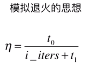
理解

模拟退火的思想

代码实现

def dJ_sgd(theta, x_b_i, y_i):
    return x_b.T.dot(x_b.dot(theta) - y_i) * 2

def sgd(x_b, y, initial_theta, n_iters):
    t0 = 5
    t1 = 50
    
    def learning_rate(t):
        return t0/(t+t1)
    
    theta = initial_theta
    for cur_iter in range(n_iters):
        rand_i = np.random.randint(len(x_b))
        gradinet = dJ_sgd(theta,x_b[rand_i],y[rand_i])
        theta = theta - learning_rate(cur_iter) * gradinet
    
    return theta

%%time
x_b = np.hstack([np.ones((len(x), 1)) ,x])
initial_theta = np.zeros(x_b.shape[1])
theta = sgd(x_b, y, initial_theta,n_iters=len(x_b)//3)
>>>Wall time: 110 ms

使用sklearn中的SGD方法

只能解决线性模型

from sklearn.linear_model import SGDRegressor 

sgd_reg = SGDRegressor()

%time sgd_reg.fit(x_train_standard,y_train)

sgd_reg.score(x_test_standard,y_test)

>>>Wall time: 260 ms
	0.7938286715532883

7，关于梯度调试

图示及公式理解

代码实现
先创建一组数据以供给使用

np.random.seed(666)
x = np.random.random(size=(1000,10))

true_theta = np.arange(1,12,dtype=float)

x_b = np.hstack([np.ones((len(x),1)),x])
y = x_b.dot(true_theta) + np.random.normal(size=1000)

def J(theta, x_b, y):
    try:
        return np.sum((y - x_b.dot(theta))**2) / len(x_b)
    except:
        return float('inf')

def dJ_math(theta, x_b, y):
    return x_b.T.dot(x_b.dot(theta) - y) * 2. / len(x_b)

def dJ_debug(theta, x_b, y, epsilon=0.01):
    res = np.empty(len(theta))
    for i in range(len(theta)):
        theta_1 = theta.copy()
        theta_1[i] += epsilon
        theta_2 = theta.copy()
        theta_2[i] -= epsilon
        res[i] = (J(theta_1, x_b, y) - J(theta_2, x_b, y)) / (2*epsilon)
    return res

def gradinet_descent(dJ, x_b, y, initial_theta, eta, n_iters = 100, epsilon=1e-8):
    
    theta = initial_theta
    i_iters = 0
    
    while i_iters < n_iters:
        gradient = dJ(theta, x_b, y)
        last_theat = theta
        theta = theta - eta * gradient

        if (abs(J(theta, x_b, y) - J(last_theat, x_b, y)) < epsilon):
            break
            
        i_iters += 1
        
    return theta

使用

x_b = np.hstack([np.ones((len(x),1)),x])
initial_theta = np.zeros(x_b.shape[1])
eta = 0.01

%time theta = gradinet_descent(dJ_debug, x_b, y, initial_theta, eta)
>>>Wall time: 50 ms

8，总结

批量梯度下降法

需要对每一个数据进行梯度下降
优点：稳定，一定可以向损失函数下降最快的方向前进
缺点：速度慢，在每一次都需要对所有的样本看一遍

随机梯度下降法

每次只看一个样本
优点：速度快，每次只看一个样本
缺点：不稳定，每一次的方向是不确定的（有可能相反方向前进）
关于随机↓

小批量梯度下降法

综合上边的优点，每次看 k 个样本
例如：一次看10个样本
相对灵活的取值